Synthetic Data in Healthcare:
A Focus on EEG Signals
Addressing class imbalance in seizure detection by synthesizing realistic ictal EEG with generative models - GAN, VAE, and Diffusion - trained on the CHB-MIT Scalp EEG Database.
The Problem
Epilepsy affects over 50 million people worldwide. Automated seizure detection from scalp EEG could enable real-time monitoring, but two obstacles make it unreliable: clinical data scarcity (patient recordings are expensive, require expert annotation, and are restricted by privacy and regulatory constraints) and extreme class imbalance (seizure activity accounts for less than 0.4% of recording time). EEG signals are further complicated by strong inter-subject variability, non-stationarity, and noise - making cross-patient generalization particularly difficult.
This thesis investigates whether synthetic data augmentation using generative models (TimeGAN, CVAE, LDM) can address these problems - but augmentation is not guaranteed to help. It could reduce subject-dependent overfitting by increasing training variability, or it could amplify subject-specific patterns if the generator reproduces them. Under a strict LOPO protocol, this work tests which outcome prevails and seeks to distinguish genuine gains from misleading improvements.
Methodology
Research questions, evaluation strategy, and literature gaps
Dataset
CHB-MIT Scalp EEG: patient profiles, recordings, and seizure distribution
Data Pipeline
Cleaning, filtering, windowing, caching, and parameter justifications
Generative Models
TimeGAN, CVAE, LDM: architectures, design decisions, and trade-offs
Roadmap
7 experiments (E1–E7), timeline, and protocol rules
Status
Implementation progress and what's left
Results
LOPO and single-split experiment results (E1-E5)
Glossary
Key terms and acronyms used throughout the thesis
References
All cited works, organized by source type
Methodology
Research framework, questions, and evaluation strategy
Goals
Research Questions
CRISP-DM Framework
This thesis follows the CRISP-DM methodology, chosen for its structured, iterative approach to data-driven research. Unlike purely linear workflows, CRISP-DM explicitly supports feedback loops between phases - for example, evaluation results may reveal the need for different preprocessing, looping back to Data Preparation. The six phases map to thesis chapters as follows:
*Deployment is adapted for academic context: rather than production deployment, Chapter 6 covers conclusions, practical recommendations (RQ5), and directions for future clinical integration.
Evaluation Strategy
All experiments use LOPO cross-validation (23 folds, one patient held out completely per fold) with a frozen 1D-CNN detector. Synthetic data enters training only - never validation or test. The model never sees any test patient data during training, normalisation, or generation.
Systematic Literature Review (26 Articles) RQ1
Conducted following PRISMA guidelines across IEEE Xplore, PubMed, Scopus, and Web of Science. Inclusion criteria: synthetic data generation or augmentation for healthcare time-series, published 2020–2025.
What's Being Evaluated: The Generators, Not the Classifier
The detector is a measuring instrument - it's frozen specifically so it can't be the source of any performance difference. The actual object of study is the synthetic data itself. Four complementary goals (thesis Section 4.4), structured so the data is evaluated directly before it ever touches the downstream classifier:
Fidelity and discriminability evaluate the synthetic data with no dependence on the downstream task. Utility uses the frozen detector as an indirect measurement of data quality. Subject-identity analysis checks for memorisation and privacy risks - whether synthetic data makes patients more identifiable rather than less. Together they answer "is this synthetic data any good?" from multiple angles - the classifier result alone would be insufficient.
Single-split fidelity results (all generators, 3 seeds) are available on the Results page. Full LOPO fidelity, utility, and subject-identity results follow once E2-E5 LOPO completes.
Complete Metrics Reference
Every metric in the thesis evaluation framework, grouped by what it evaluates. The "Why?" column traces each choice to its source - a literature gap, an SLR finding, or a methodological requirement.
Computed per experiment Computed post-hoc from LOPO results Computed in E7 (after E3-E5 LOPO)
Utility - Does synthetic data improve seizure detection?
| Metric | What it answers | Why this metric? |
|---|---|---|
| AUPRC (primary) | Overall detection quality across all thresholds, sensitive to rare-class performance | A model predicting "no seizure" always gets ~99.6% accuracy and decent AUROC, but terrible AUPRC. Precision-recall curves are more informative than ROC curves for imbalanced problems (Saito & Rehmsmeier, 2015). Already used in seizure detection: Yuan et al., 2019; Constantino et al., 2021; Manzouri et al., 2022; Yamada et al., 2025; Park et al., 2026. |
| AUROC | Overall discrimination (threshold-independent), regardless of class balance | Enables comparison with prior seizure detection literature. Standard metric in Bing et al., 2022 (TSTR evaluation uses AUROC) and commonly reported in clinical EEG studies. Not primary because it's insensitive to class imbalance (Saito & Rehmsmeier, 2015). |
| F1 (optimal threshold) | Best achievable precision-recall balance. Sweeps all thresholds and reports the maximum F1, not F1 at the default 0.5 cutoff | Ghanem et al., 2023: "F1 is particularly useful with imbalanced classes" (harmonic mean penalises both false positives and false negatives). They also recommend threshold optimization for imbalanced classification: "selecting the threshold with the best performance" rather than defaulting to 0.5. With <1% seizure prevalence, the model may output well-calibrated but low probabilities for real seizures - fixed 0.5 would misclassify them all. We report both the max F1 and the threshold that achieves it. F1 is a standard downstream metric for EEG generation (You et al., 2025, Table 2; Zhao et al., 2022). |
| Sensitivity @ 95% Specificity | How many seizures are caught when false alarm rate is clinically acceptable (5%) | Chua et al., 2022 report sensitivity "at >95% specificity" on CHB-MIT as their primary operating-point metric for seizure detection. Baumgartner & Koren, 2018: "Low false-positive alarm rates are of critical importance for acceptance of algorithms in a clinical setting." At 95% specificity, the system fires at most 1 false alarm per 20 interictal windows - a widely adopted clinical threshold in medical binary classification. |
| Per-patient AUPRC (mean/std) | Whether utility is consistent across patients or driven by a few easy cases | Global AUPRC can be inflated by a few high-seizure patients. Per-patient dispersion reveals stability across the cohort (Zhao et al., 2022). |
| TSTR AUPRC | Can a detector trained on only synthetic seizures still detect real ones? | Isolates generator quality from augmentation effects. If TSTR fails, synthetic data lacks seizure-discriminative structure regardless of ratio. Used by Bing et al., 2022. |
| Wilcoxon signed-rank p-value | Is the improvement statistically significant across all 23 patients? | Non-parametric (no normality assumption). 23 paired LOPO observations. Standard for comparing paired fold results when normality cannot be assumed. |
Fidelity - Does synthetic data look like real EEG?
| Metric | What it answers | Why this metric? | ||||||||||||||||||||||||
|---|---|---|---|---|---|---|---|---|---|---|---|---|---|---|---|---|---|---|---|---|---|---|---|---|---|---|
| PSD per frequency band | Does synthetic EEG have the same spectral shape (delta/ theta/ alpha/ beta/ gamma)? | Carrle et al., 2023 showed GANs smooth spectral peaks - spectral fidelity is the first thing to check. You et al., 2025 lists PSD as a standard generative quality metric (Table 3). Addresses RQ1, RQ5 - utility is frequently assessed, but time-series realism is not always tested directly. | ||||||||||||||||||||||||
| KL divergence per band | Quantifies how far synthetic spectral distribution is from real, per band | A scalar summary of PSD difference per band - makes cross-generator comparison possible (PSD plots are visual, KL is a number). Standard in distribution matching. | ||||||||||||||||||||||||
| C2ST (discriminative score) | Can a classifier tell real from synthetic? (50% = indistinguishable) | Tests the joint distribution (all features together), not just marginals. Introduced with TimeGAN (Yoon et al., 2019); applied to health sensors by Lange et al., 2024. | ||||||||||||||||||||||||
| Autocorrelation | Are temporal dependencies (how one time point relates to the next) preserved? | Lin et al., 2020 compute MSE between real and synthetic autocorrelation functions as a primary fidelity metric (Table 3), showing that temporal dependency preservation is essential for realistic time-series generation. A generator producing correct spectra but shuffled temporal structure would pass PSD but fail autocorrelation - the two are complementary. | ||||||||||||||||||||||||
| Cross-channel correlation | Are spatial relationships between EEG channels preserved? | Seyfi et al., 2022 compute MAE between real and synthetic correlation matrices "for each pair of channels in the EEG dataset" and show that preserving inter-channel correlations is essential for realistic multi-channel generation. Lange et al., 2024 compare Pearson correlation between signals as a quality metric for synthetic health sensor data. | ||||||||||||||||||||||||
| Amplitude distributions | Are overall signal amplitudes realistic? | Lange et al., 2024 explicitly compare "the distribution density of signal values" between real and synthetic data via histograms as a core quality metric. You et al., 2025 Table 3 lists amplitude-level metrics (ABA) among generative quality measures. Histogram + Q-Q plot catch both global scale drift and distributional shape mismatch. | ||||||||||||||||||||||||
| t-SNE embedding | Do synthetic samples overlap with real data in feature space, or cluster separately? | Visual complement to C2ST. Reveals mode collapse (synthetic data clusters in one region) or mode dropping (some real patterns never generated). Not a scalar metric - for qualitative interpretation. | ||||||||||||||||||||||||
Excluded metrics and selection principlesThe literature reports dozens of fidelity metrics for synthetic data (You et al., 2025, Tables 2-3; Ibrahim et al., 2025, Section 2.3). We select metrics based on three principles, validated against adoption patterns across our 26-paper corpus (17 primary studies, 9 reviews):
The key insight: most metrics reported in EEG generation reviews (You et al., 2025; Carrle et al., 2023) originate in either paired settings (autoencoder/denoising) or image modalities. Neither applies to our unconditional class-conditional EEG generators. Our suite is designed for unpaired distributional evaluation of 1D multi-channel time-series generators, targeting the specific properties that matter for EEG: spectral shape, temporal structure, and inter-channel coupling. Notable: the dominant utility metric in EEG generation papers is accuracy (12/17 primary studies, e.g. Ahuja et al., 2024; Boukhennoufa et al., 2023; Sobhani et al., 2025; Waters et al., 2024), which is uninformative at <1% seizure prevalence. AUPRC appears in 0/26 SLR papers - however, it is established in the broader seizure detection literature (Yuan et al., 2019; Constantino et al., 2021; Manzouri et al., 2022; Yamada et al., 2025; Park et al., 2026), with theoretical justification in Saito & Rehmsmeier, 2015. Adopting it in the EEG generation context is a gap-filling contribution. |
||||||||||||||||||||||||||
Privacy/ Memorisation - Is the generator copying patients?
| Metric | What it answers | Why this metric? |
|---|---|---|
| Subject-ID linear probe accuracy | Can a classifier recover which patient the data came from? High accuracy = memorisation risk | If a generator memorises patient-specific signatures, "synthetic" data is really patient data with extra steps - defeating the privacy purpose. Motivated by You et al., 2025 and Gonzales et al., 2023 - privacy and memorisation risks are rarely evaluated alongside utility (RQ4). |
| k-NN proximity (synth→real) | How close are synthetic samples to their nearest real neighbors in embedding space? | Complements the linear probe: even if patient ID isn't explicitly recoverable, synthetic samples that sit on top of real ones may be near-copies. Operates in cosine distance on frozen detector embeddings. |
| Proximity ratio | synth-to-real distance / real-to-real distance. Below 1.0 = suspicious closeness | Normalises proximity against a baseline. Real data naturally has some self-similarity - the question is whether synthetic data is closer than real data is to itself. A thesis-specific contribution (no standard benchmark exists for EEG proximity). |
| Excluded: Membership inference | - | Tests if an adversary can tell whether a specific sample was in the training set. Requires a shadow-model training loop and assumes the attacker has access to auxiliary data from the same distribution. Our subject-ID probe addresses a different and more domain-relevant question: not "was this in training?" but "which patient did this come from?" - because in LOPO, the sensitive attribute is patient identity, not dataset membership. Re-identification is a distinct privacy risk from membership inference (Ibrahim et al., 2025, Section 2.3). Our k-NN proximity ratio complements this by detecting near-copies without requiring shadow models. |
| Excluded: Differential privacy (DP-SGD) | - | Provides formal mathematical privacy guarantees by adding calibrated noise during training. Excluded because: (1) formal DP requires a privacy budget (epsilon) chosen a priori, adding a hyperparameter orthogonal to our research questions; (2) the privacy-utility tradeoff means DP-trained generators produce lower-quality synthetic data (Ibrahim et al., 2025: "underscoring the often-present trade-off between privacy and utility"), confounding the comparison of generator architectures; (3) our research questions ask whether generators memorise, not whether we can prevent it - that is a separate engineering decision downstream of results. |
Efficiency - Is the improvement worth the compute?
| Metric | What it answers | Why this metric? |
|---|---|---|
| AUPRC gain over baseline | How much better than real-only training (E1)? | The denominator for cost-benefit. Without a gain, there is no benefit to justify any cost. Computed from aggregated LOPO results. |
| Total time (train + generate) | How many GPU-hours does the full pipeline cost? | Practical concern: a generator that takes 100h for +0.01 AUPRC is not viable in a clinical setting. Epoch times are recorded per fold during training and aggregated in E6. |
| Gain per hour | AUPRC improvement normalised by total compute time | Ranks generators by bang-for-buck. A simpler model with modest gains may be more practical than a complex one with marginal extra improvement - a finding echoed by the broader augmentation literature (see Carrle et al., 2023 on diminishing returns). Part of E6 cross-generator analysis. |
| Diminishing returns flag | Does adding more synthetic data (higher ratio) start hurting performance? | Carrle et al., 2023 found gains plateau or reverse beyond 100% (r=-0.37 between baseline accuracy and augmentation benefit). Detects "too much synthetic" degradation. |
Why all four axes? Utility alone is insufficient: a generator could improve AUPRC by memorising patients (fails privacy), produce high-scoring but spectrally unrealistic signals (fails fidelity), or require impractical compute (fails efficiency). This multi-axis approach directly addresses SLR Gaps 3 and 6 - most prior EEG augmentation work only reports utility (Boukhennoufa et al., 2023; You et al., 2025).
Implementation status: Utility and fidelity metrics run automatically per experiment. Privacy analysis (E7) and efficiency analysis (E6 post-hoc) are fully implemented but will execute once the LOPO evaluation completes for all generators - they need cross-experiment data to produce meaningful comparisons.
Research Gaps Identified in the SLR
These gaps directly motivate the experimental design and research questions:
CHB-MIT Scalp EEG Database
Boston Children's Hospital/ MIT · PhysioNet v1.0.0 (2009) · 23 unique subjects across 24 cases with intractable epilepsy
Re-Recording: chb01 = chb21
chb21 was recorded 1.5 years after chb01, from the same female subject. This is the only re-recording in the dataset. For train/test splitting, chb01 and chb21 must always stay on the same side of any patient-level split.
The original database was published in 2009. chb24 was added in December 2010 and is absent from SUBJECT-INFO (no gender or age on record). Total: 24 cases from 23 unique subjects - 5 males, 17 females, 1 unknown.
Recordings per Patient
Non-seizure and seizure files stacked per patient case
Patient Age Distribution
Ages range from 1.5 to 22 years (pediatric cohort)
Gender Distribution
17 females, 5 males; chb24 has no gender/age on record
Patient Profiles
24 cases from 23 unique subjects. chb21 highlighted as the only re-recording.
| Patient | Gender | Age | Files | Seizure | % |
|---|
Data Pipeline
From raw EDF files to normalized, windowed tensors. Covers cleaning, signal preprocessing, windowing, caching, and parameter justifications.
Phase 1: EDF Cleaning
Homogenization of raw CHB-MIT EDF files into clean, standardized EDF+ format
Cleaning Pipeline (homogenize.py)
Cleaning Results
Channels Removed
Key Challenges Solved
TARGET_MONTAGE). Missing channels zero-padded; extra channels dropped. QC rejects windows with flat (zero-padded) channels.Output: Standard 10-20 Bipolar Montage (23 channels)
The 23 bipolar channels retained after removing non-EEG channels and resolving duplicates.
Per-Patient Cleaning Summary
What the homogenization pipeline actually did to each case. Colour legend: ● stable montage ● montage split required ● non-EEG channels removed.
| Case | Montage | Channels Removed | Action taken |
|---|
Phase 2: Signal Preprocessing
Literature-grounded preprocessing pipeline applied to the homogenized EEG signals before windowing and model training
Why Preprocess?
Raw scalp EEG is full of things that aren't brain signals: powerline hum at 60 Hz, slow drifts from electrode chemistry, muscle noise from jaw clenching or eye movements, and the occasional electrode pop when something shifts. If generators train on this raw signal, they learn to reproduce artefacts alongside real neural patterns - and the synthetic data inherits those artefacts (Carrle et al., 2023). The pipeline below cleans the signal while keeping all the clinically relevant information, and it's applied consistently across all experiments so comparisons are fair.
Importantly, normalisation parameters come from training data only. This prevents information about test patients from leaking into the pipeline.
Preprocessing Pipeline (applied after homogenization, before windowing)
data/loader.py)scipy.signal.iirnotch, Q=30Powerline interference is an environmental, non-biological artefact caused by electromagnetic fields from the electrical mains supply. In the United States (where the CHB-MIT recordings were made at Boston Children’s Hospital), the mains frequency is 60 Hz. This interference couples capacitively and inductively into the electrode leads and amplifier circuits, producing a sustained sinusoidal component at 60 Hz and its harmonics (120 Hz, 180 Hz, etc.) that is superimposed on the genuine neural signal.
Sobhani et al., 2025 explicitly identify power-line interference as one of the noise sources in raw EEG: “A variety of noise and artifacts, including power-line interference, eye movements, and muscle activity, are commonly present in raw EEG recordings.”
The 60 Hz line noise falls squarely in the gamma band (30–100+ Hz). If left unremoved, it contaminates power spectral density estimates, distorts differential entropy features in that range, and - critically - may cause classifiers to learn the mains peak as a spurious feature rather than genuine neural activity. Carrle et al., 2023 note that even generative models can reproduce or fail to reproduce the 50 Hz line noise artefact, directly demonstrating that it is a persistent, recognisable feature of real recordings: “Figure 5 in the study of Bird et al. (2021) demonstrates highly smoothed versions of the 50 Hz line noise artifact as well as the absence of alpha peaks in the synthetic data produced with a GPT model.”
Our bandpass filter (0.5–40 Hz) already attenuates frequencies above 40 Hz, which would remove 60 Hz content. However, the rolloff of a 4th-order Butterworth is gradual, not brick-wall: at 60 Hz the attenuation is only ~24 dB. Powerline interference can be 10–100× stronger than neural signals, so partial attenuation may not suffice. The notch filter surgically removes a narrow band around exactly 60 Hz (and 120 Hz) with minimal disturbance to adjacent frequencies. Sobhani et al., 2025 suggest that “environmental artifacts may be avoided using a band filter since their frequency differs from the EEG signals of interest.” We apply both: notch first (surgical removal of the known contaminant), then bandpass (broader spectral shaping).
- Frequencies: 60 Hz (US mains fundamental) + 120 Hz (2nd harmonic). Higher harmonics (180, 240 Hz) fall well outside our 0.5–40 Hz bandpass and need not be explicitly notched.
- Quality factor Q=30: Produces a notch ~2 Hz wide at the −3 dB points. This is narrow enough to preserve neural gamma activity at 58 Hz and 62 Hz while fully attenuating the mains peak.
- Filter type: IIR notch (
scipy.signal.iirnotch) applied withfiltfiltfor zero-phase response, preserving the temporal alignment of seizure onsets.
scipy.signal.iirnotch(60, 30, 256) + scipy.signal.filtfilt, applied per channel. Repeated for 120 Hz.filtfilt)Raw EEG contains spectral content from DC (0 Hz) up to the Nyquist frequency (128 Hz at our 256 Hz sampling rate). Much of this is not neural. Below ~0.5 Hz, the signal is dominated by slow electrode drift - voltage changes caused by electrochemical reactions at the electrode-skin interface, sweat-related impedance fluctuations, and patient movement. Above ~40–70 Hz, the dominant source is electromyographic (EMG) contamination from scalp, facial, and neck muscles, which produces broadband high-frequency energy that can be orders of magnitude larger than neural gamma activity.
Sobhani et al., 2025 describe this directly: “The FIR filter in our context was made to allow signals between 0.3 and 70 Hz, which removes high-frequency muscular distortions and slow DC drifts while keeping the frequency range that is most important for clinical and cognitive EEG studies.”
You et al., 2025 warn unambiguously: “Without adequate preprocessing and filtering strategies, such artifacts may introduce substantial variability and degrade the reliability of feature extraction and classification.”
Their review also observes that despite claims of working with “raw” EEG, most deep learning models still depend on filtered data: “Although many deep learning models claim to work with raw EEG signals, in practice, they still heavily depend on preprocessed data, such as artifact removal and band-pass filtering, limiting their adaptability in unstructured environments.”
Without filtering, DC drift can saturate the input dynamic range of downstream models. EMG contamination above 40 Hz overwhelms neural gamma activity. Frequency-domain features (PSD, band power, differential entropy) become unreliable because they measure noise rather than brain activity. Classifiers trained on unfiltered data learn artefact patterns rather than neural patterns, producing results that do not generalise.
This range retains the five clinically relevant EEG bands (delta through low gamma) while excluding both DC drift and muscle contamination. The choice is well-supported by the SLR literature:
Our lower cutoff of 0.5 Hz (rather than 1 Hz as in Carrle et al., 2023) preserves the full delta band, which is relevant for seizure detection in paediatric patients where slow-wave abnormalities are common.
filtfilt, not FIRSobhani et al., 2025 advocate for FIR filters because of their “linear phase properties, which guarantee that the temporal structure of the EEG waveforms is maintained without introducing phase distortion.” This is valid for a causal (real-time) filter. However, we apply filtfilt (forward-backward filtering), which makes any IIR filter zero-phase - achieving the same temporal-structure preservation as FIR while requiring a much lower filter order (4th-order Butterworth vs. typically 100+ order FIR for a comparable transition band). Lower order means fewer edge artefacts and faster computation across 683 files × 23 channels.
scipy.signal.butter(N=4, Wn=[0.5, 40], btype='band', fs=256) + scipy.signal.filtfilt. Zero-phase; no temporal distortion.np.clip after filteringEven after notch and bandpass filtering, the signal may contain transient, high-amplitude artefacts: electrode pops (sudden impedance changes), large body movements, or electrical interference spikes. These events produce amplitudes far exceeding normal EEG (±100–200 µV) and even ictal activity (±300–500 µV). Leaving them unchecked distorts the variance and mean of the signal, corrupts normalization statistics, and forces downstream models to waste capacity modelling extreme outliers.
The literature presents two competing approaches to handling artefacted segments:
Clipping is a softer alternative that resolves this tension: it bounds the outlier without discarding the window. A brief electrode pop that produces a 2000 µV spike in 50 samples out of 1024 is clipped to ±800 µV, preserving the remaining 974 samples of genuine signal. The window stays in the training set, avoiding the data loss and exclusion bias that Dakshit et al., 2023 warns about.
The threshold is chosen to be well above physiological amplitudes while catching clearly non-neural outliers:
- Normal awake EEG: ±50–200 µV
- Ictal (seizure) activity: ±200–500 µV
- Our clipping threshold: ±800 µV - leaves a wide margin above seizure amplitudes
- Electrode pops/ movement artefacts: can reach ±2000–5000 µV
This means genuine neural signal (including large seizure discharges) is never clipped, while transient artefacts are bounded to a range where they cause minimal distortion to downstream statistics.
np.clip(signal, -800, 800) - applied per channel after filtering, before normalisation.EEG amplitude varies dramatically across subjects (due to skull thickness, electrode impedance, scalp conductivity), across channels (due to electrode placement and reference scheme), and across recording sessions. Without normalisation, a classifier may learn to distinguish patients by their absolute amplitude - a subject signature rather than a seizure signature. Carrle et al., 2023 and You et al., 2025 identify this as a core risk: models may unintentionally learn subject-dependent patterns instead of signal characteristics that transfer across individuals.
The literature uses both approaches, but for different reasons:
tanh output. They warn about a crucial subtlety: “For many (clinical) applications, the relative signal strength across electrodes is meaningful... These differences should therefore not be factored out by, e.g., normalizing the channels individually.”We use per-channel z-score (mean=0, std=1) because it standardises scale without bounding the range, which is important for preserving the relative amplitude of seizure events (which can be 3–5σ deviations - exactly the kind of outlier a classifier needs to detect). Min-max [−1, 1] would compress seizure spikes into the same range as baseline activity.
Normalisation parameters (mean, std per channel) are learned statistics. If computed on the full dataset (including validation and test subjects), they leak information about the test distribution into the training pipeline. All preprocessing steps that learn parameters must therefore be fit using training data only.
You et al., 2025 highlight this as a widespread problem: evaluation protocols are often underspecified, and leakage risk is high. Reported improvements can strongly depend on how data is split and how synthetic samples enter the pipeline. When subjects appear in both training and testing, or when preprocessing is fitted beyond the training set, results can look strong without reflecting true generalization.
You et al., 2025 confirm this as a known problem across the EEG generation literature, and the entire thesis evaluation framework (G2, RQ5) is built around preventing this type of leakage.
norm_params_{hash}.npz (keyed by training case list to prevent cross-fold leakage); applied as (x − μ)/ σ. Already implemented in data/loader.py.Clipping handles transient amplitude spikes, but two classes of unusable windows remain:
- Flat (zero-padded) channels. The homogenization step fills missing or removed channels with zeros to maintain the 23-channel matrix shape. A window where an entire channel is zero has no neural information in that channel and would bias the model toward learning that zero=normal.
- Saturated windows. If a large artefact pushed >25% of samples in a channel to the ±800 µV clip boundary, the window is more artefact than signal. Unlike a brief spike (clipped and contained), a sustained saturation means the true signal is irrecoverably lost for that window.
If any channel’s standard deviation < 0.01 µV across the entire window, the window is rejected. This catches zero-padded channels from homogenization and dead electrodes.
If >25% of samples in any channel are at the ±800 µV clip boundary, the window is rejected. This catches sustained artefacts where the true signal is irrecoverable.
Design Decision: No ICA-Based Artefact Removal
Independent Component Analysis decomposes multichannel EEG into statistically independent sources. Some components correspond to neural activity; others correspond to artefacts (eye blinks, muscle, cardiac). By identifying and removing artefact components and reconstructing the signal, ICA can dramatically improve signal-to-noise ratio.
Sobhani et al., 2025 provide a strong justification for ICA in their emotion-recognition pipeline: “By breaking down the EEG signals into statistically independent components, ICA makes it possible to identify and eliminate artifact-related components. ICA greatly increases the signal-to-noise ratio and strengthens the stability of features recovered using DWT.”
Carrle et al., 2023 use automated ICA via ICLabel, which classifies each component as brain, muscle, eye, heart, line noise, channel noise, or other - removing the need for manual inspection.
Despite its benefits, ICA is not appropriate for every setting. We deliberately omit it for four reasons, each grounded in the literature or the experimental protocol:
ICA computes a mixing matrix from the full recording. If this decomposition is fitted on data that includes test subjects (even indirectly, through shared statistics), it leaks information about the test distribution into training. Since all preprocessing steps that learn parameters must be fit using training data only, running ICA per-patient per-fold would be required - adding significant computational overhead (683 files × 23 LOPO folds) for marginal benefit on long-term monitoring data.
The patients were paediatric epilepsy cases undergoing long-term video-EEG monitoring in a hospital setting, often sedated or sleeping. Eye-blink artefacts (the primary target of ICA) and voluntary muscle artefacts are far less prevalent than in awake BCI or emotion-recognition paradigms. Zhao et al., 2022 and Chaibi et al., 2024 work with intracranial EEG and do not use ICA at all, relying on simpler filtering and expert segment selection.
The core thesis question is whether synthetic augmentation helps on unseen subjects. If the generator is trained on aggressively cleaned data, it synthesises signals that lack the noise characteristics of real EEG. When these synthetic samples are mixed with real (uncleaned) data for downstream evaluation, the distribution mismatch can reduce robustness rather than improve it. You et al., 2025 observe that models operating in real-world conditions must handle “high noise, dynamic variability, and low signal-to-noise ratios” - over-cleaning the training data undermines this goal.
CHB-MIT has 23 channels after homogenization. While this is above the minimum for ICA (Sobhani et al., 2025 use 8 channels), reliable component separation improves with channel count. They set n_components = 8 (equal to their channel count), and their success is partly due to the targeted 8-channel montage. With 23 channels across the full scalp, the number of mixed sources is larger and component identification is less clearcut, especially for automated methods without manual verification.
EEG Frequency Bands Retained (0.5–40 Hz)
The bandpass filter preserves five clinically relevant frequency bands. Seizure activity in scalp EEG is concentrated in theta and alpha ranges, with ictal rhythmic discharges typically manifesting as evolving theta (3–7 Hz) activity.
Design Decisions
Every parameter is either grounded in the literature (indicated by inline citations) or is an implementation decision where the literature does not prescribe a specific value (indicated as project-specific in the justification).
Framework & Tooling
filtfilt for zero-phase filtering, Welch PSD estimation. Standard DSP tools with no reason to reimplement.Data Caching & Memory Management
The dataset after preprocessing is ~43 GB. Pre-computing all overlapping windows would nearly double that (each sample appears in two windows with 50% overlap), exceeding both the 32 GB RAM and available disk. The approach below isn't just an optimisation - it's the only way to run experiments on this hardware at all.
| Decision | Choice | Justification |
|---|---|---|
| Cache format | Flat preprocessed signals, not pre-windowed arrays | With 50% overlap, each sample appears in two windows, inflating ~43 GB to 64–74 GB. Storing the flat signal instead and computing windows on the fly via signal[:, start:start+1024] eliminates this duplication. Total cache: ~35–40 GB (∼40% less). |
| Signal cache format | <case>_signals.npy + <case>_index.npz |
Per case: one uncompressed .npy file (23 × N samples, float16) for memory mapping, plus a small compressed .npz index (~100 KB) with precomputed valid window start positions, labels, patient ID, and QC rejection count. The signal files use .npy (not compressed .npz) because numpy’s mmap_mode='r' requires an uncompressed format - compressed archives must be fully decompressed into RAM before access, defeating the purpose of memory mapping. The index files are small enough (~100 KB) to load entirely, so they use compressed .npz to save disk space. |
| Synthetic window storage | Compressed .npz files |
Generator outputs (E3–E5) are saved as synthetic_ratio_<r>.npz containing windows, labels, and patient IDs. Unlike signal caches, synthetic windows are small (~4–5K windows per seed) and loaded fully into RAM at training time - no memory mapping needed. Compressed .npz is used for reproducibility (the exact same windows are reused across detector training runs) and auditability (files can be inspected in notebooks for quality checks). |
| Memory strategy | Memory-mapped I/O (mmap_mode='r') |
Cannot load 35–40 GB into 32 GB RAM. Memory mapping lets the OS page cache manage which signal pages are resident. Python heap stays under ~10 MB (index arrays only). Each __getitem__ reads ~46 KB from disk via the page cache. |
| Numeric precision | float16 on disk, float32 at access time | Halves disk and mmap footprint. EEG values after clipping are in [−800, +800] µV - well within float16 range (up to 2048.0 exact). Quantization error (~0.01–0.1 µV) is below the EEG noise floor (~1–5 µV). Cast to float32 in __getitem__ before normalization and training. |
| QC timing | Precomputed at cache-build time | QC costs ~303 µs/window. With ~1.4M windows × ~10 epochs, on-the-fly QC would add ~70 min/experiment. Precomputing during the one-time cache build amortizes this entirely. QC runs on preprocessed signals before normalization (thresholds are in µV). |
| Normalization timing | On the fly in __getitem__ |
Normalization params depend on the training set of each LOPO fold. Pre-normalizing would require 23 copies of the cache. Instead, caches store raw µV values and normalization is applied per window (~37 µs overhead). Total per-window cost: ~60–70 µs - negligible vs ~1–2 ms GPU compute per batch element. |
| Cross-file windows | Prevented (windows respect file boundaries) | The flat signal concatenates multiple EDF files per case. Windows are enumerated within each file independently, so no window spans a recording boundary (which could be hours or days apart). Data loss: at most 1023 samples (~4s) per file. |
| Batch sampling | Case-aware (grouped by patient) | With 24 memory-mapped files, pure random shuffling thrashes the OS page cache (each case is 1–4 GB). CaseAwareSampler groups windows by case within each epoch - case order and within-case order are both shuffled, so every window is seen once per epoch in a valid permutation, but consecutive batches hit the same mmap file. This maximizes page cache hits without affecting training dynamics. |
| Mmap cache size | LRU, max 4 open files | Keeping all 24 mmaps open wastes page table entries under memory pressure. An LRU cache of 4 open files provides headroom for batch boundaries while keeping the virtual memory footprint bounded. Combined with case-aware sampling, the active case is nearly always cached. |
Hardware context: Target machine has 32 GB RAM, ~98 GB disk (shared with OS and Python env), and an RTX 3080 Ti (12 GB VRAM). A naive pre-windowed loader consumed ~125 GB RAM and was OOM-killed on first training attempt. The flat-signal approach reduces disk to ~35–40 GB and RAM to ~10 MB.
Generator & oversampling memory: CVAE and LDM training keep data tensors on CPU and move per-batch to GPU (12 GB VRAM cannot hold the full ictal set + model + optimizer). SMOTE/ADASYN subsample interictal windows to 5× ictal count before oversampling (reduced from 10× after OOM failures in LOPO) - without this, the flattened feature matrix would exceed available RAM.
Preprocessing Parameters
Canonical definitions and literature backing: Notch filter, Bandpass filter, Amplitude clipping, Normalization.
| Parameter | Value | Justification |
|---|---|---|
| Notch filter | 60 Hz + 120 Hz, Q=30 | US mains frequency - CHB-MIT recorded at Boston Children's Hospital. Q=30 gives ~2 Hz notch width, narrow enough to remove interference without eating into the EEG signal. Standard across EEG pipelines (You et al., 2025). |
| Bandpass | 0.5–40 Hz | Carrle et al., 2023 used 1–40 Hz; lower cutoff reduced to 0.5 Hz to preserve full delta band, relevant for pediatric seizure detection where slow-wave abnormalities are common. No useful neural signal above 40 Hz in scalp EEG after filtering. |
| Filter type | 4th-order Butterworth, zero-phase (filtfilt) |
Sobhani et al., 2025 advocates FIR for linear phase, but filtfilt makes IIR zero-phase at lower computational cost. Tradeoff documented in thesis Section 4.3. Zero-phase is essential to avoid shifting seizure onset timing. |
| Amplitude clipping | ±800 µV | Normal EEG: ±50–200 µV. Ictal: ±200–500 µV. Electrode pops: ±2000+ µV. 800 keeps seizures intact while bounding artifacts. Softer than outright rejection - avoids exclusion bias (Dakshit et al., 2023). |
| Normalization | Per-channel z-score (train-only) | Z-score is the most common normalization for EEG classification pipelines (You et al., 2025). Parameters hash-keyed per LOPO fold to prevent leakage - thesis Section 1.4 mandates this. |
Windowing Parameters
See also: Window QC criteria and frequency bands retained.
| Parameter | Value | Justification |
|---|---|---|
| Window size | 4s = 1024 samples | Carrle et al., 2023. Zhao et al., 2022 used 10s, but 4s gives more windows (important for class balance). Long enough to capture seizure rhythmic patterns (2–10s evolution). |
| Overlap | 50% (512-sample step) | Prevents seizures on window boundaries from being missed. 50% is a standard tradeoff between coverage and redundancy in EEG sliding-window analysis. |
| Ictal threshold | ≥50% of window in seizure | Standard in the literature (Carrle et al., 2023; Zhao et al., 2022). Avoids ambiguous windows with tiny seizure fragments. |
| QC: flat channel | std < 0.01 µV | Catches zero-padded channels from homogenization and dead electrodes. Zhao et al., 2022 had clinical experts select artefact-free segments; this automates that for scalability. |
| QC: excessive clipping | >25% at ±800 µV boundary | If more than a quarter of a channel sits at the clip boundary, the window is dominated by artifact, not brain signal. Carrle et al., 2023 rejects windows with extreme amplitude stats. |
Generative Models for EEG Synthesis
A literature-grounded comparison of GAN, VAE, and Diffusion model families for synthetic ictal EEG generation. RQ1
Motivation: Why Generative Models?
In the CHB-MIT dataset, seizure windows make up roughly 0.4% of total signal time. Classical resampling (e.g. SMOTE) just interpolates between existing samples in feature space - it can't reproduce the temporal structure or spectral patterns that make real seizures look like real seizures. Deep generative models actually learn the underlying data distribution and can produce entirely new ictal segments that preserve the multi-channel dynamics, giving the detector more realistic examples to learn from.
TimeGAN adds a supervised loss that forces the generator to respect step-wise temporal dynamics - meaning each generated time point has to follow plausibly from the previous one, not just look reasonable in isolation. This solves the main weakness of vanilla GANs on time-series. It jointly trains five sub-networks (embedder, recovery, generator, discriminator, supervisor) in a shared latent space, making it the strongest GAN-family baseline for multi-channel EEG synthesis.
See Design Decisions for full parameter justifications.
A Conditional VAE (CVAE) extends the standard VAE by conditioning on a label (patient ID + class) so it can generate seizures for a specific patient on demand. The encoder compresses each 23x1024 window down to a small 128-dimensional latent vector, and the decoder rebuilds the full signal from that compressed representation. Both use 1-D convolutional layers. KL annealing prevents posterior collapse (where the model ignores the latent code and produces near-identical outputs).
Encoder/decoder reused by the LDM (E5). See Design Decisions for full parameter justifications.
Why 1-D Conv here, when TimeGAN uses GRU? The two generators have different design goals. TimeGAN uses GRU because its architecture explicitly models step-wise temporal transitions (the supervisor network enforces autoregressive dynamics). The CVAE has no such requirement - it encodes/decodes a fixed-length window in one pass. For that task, convolutional layers are faster to train, fully parallelisable, and more stable than recurrent alternatives. Carrle et al., 2023 note that CNNs are “well suited for processing biological data” due to their hierarchical structure. The tradeoff: GRU captures sequential dynamics naturally but is slow and prone to mode collapse in adversarial training; 1-D Conv captures spatial/spectral patterns efficiently but relies on the latent space (not architecture) for temporal coherence.
A Latent Diffusion Model takes the CVAE's compressed representation (the latent space) and runs the DDPM diffusion process there instead of on the full 23,552-dimensional signal. This is massively faster - denoising a 128-value latent vector is much cheaper than denoising the raw signal. It reuses the same encoder/decoder as the CVAE, so if the two models produce different quality outputs, that difference can only come from how they generate in latent space (direct sampling vs iterative denoising), not from a better encoder. The denoiser is a 1-D UNet with additive embeddings for time-step, class, and patient conditioning.
Operates in the CVAE latent space - same encoder/decoder as E4, so quality differences isolate the generation method. See Design Decisions for full parameter justifications.
Why LDM over plain DDPM? Full-resolution DDPM on 256 Hz × 23-channel windows is prohibitively slow at inference. The shared VAE latent space also enables reuse of the encoder/decoder across the CVAE and LDM, keeping the comparison controlled.
Head-to-Head Comparison
Qualitative pre-experiment assessments based on published findings in the reviewed literature, not empirical results from this thesis. Each criterion is assessed specifically in the context of multi-channel ictal EEG synthesis. Legend below explains what each criterion measures.
| Criterion (see legend) | TimeGAN | CVAE | LDM |
|---|---|---|---|
| Sample quality | High | Moderate | Very High |
| Sample diversity | Variable | Moderate | High |
| Training stability | Unstable | Stable | Stable |
| Inference speed | Fast | Fast | Slow |
| Temporal coherence | High | Moderate | High |
| Patient conditioning | Yes | Yes (label) | Yes (guided) |
| EEG literature depth | Most mature | Moderate | Growing fast |
| Mode collapse risk | High | Low | Low |
All models are evaluated using the evaluation strategy defined in the methodology.
Model Suitability Radar
Qualitative scores (1-10) for suitability to ictal EEG synthesis, derived from the literature reviewed in this thesis. These are not empirical benchmarks - they are pre-experiment assessments based on published findings, used to motivate the choice of all three models (each excels in different axes).
How scores were assigned
Sample quality & diversity: Yoon et al., 2019 show TimeGAN outperforms standard GANs on discriminative and predictive scores. Diffusion models consistently produce higher-fidelity samples than GANs/VAEs across domains (You et al., 2025). VAEs trade sharpness for stable training (Carrle et al., 2023).
Training stability: GAN adversarial training is inherently unstable (Boukhennoufa et al., 2023 address mode collapse explicitly). VAEs and diffusion use fixed loss objectives - no adversarial balancing required.
Inference speed: GANs and VAEs generate in a single forward pass. Diffusion requires iterative denoising (50-1000 steps), making it orders of magnitude slower at inference (Rouzrokh et al., 2025).
Temporal coherence: TimeGAN's supervised loss explicitly enforces step-wise temporal dynamics (Yoon et al., 2019). LDM achieves temporal coherence through iterative refinement. CVAE relies on the latent space alone, with no explicit temporal objective.
Literature depth: TimeGAN (2019) has the most EEG-specific applications. Diffusion for EEG is newer but growing rapidly (You et al., 2025; Silva et al., 2025). CVAE for EEG has moderate coverage (Pezoulas et al., 2024).
Selection Principles
The three generators form a deliberate progression from established to novel, each representing a distinct generative paradigm identified in the SLR corpus (26 papers: 17 primary studies, 9 reviews).
Excluded models and rationale
The SLR corpus contains several EEG-specific generative models. We exclude them for principled reasons, not oversight:
| Model | Source | Why excluded |
|---|---|---|
| WGAN-GP | You et al., 2025 Table 8 (Wei 2019, CHB-MIT) | TimeGAN extends the GAN paradigm with a supervised temporal embedding loss and autoencoder reconstruction loss specifically for time-series. WGAN-GP uses MLP/CNN architectures that don't model temporal dependencies explicitly - making TimeGAN the more appropriate GAN representative for sequential EEG data. Testing WGAN-GP alongside TimeGAN would compare two GAN variants rather than two generative paradigms, which is not our research question. |
| DCGAN/ DCWGAN | You et al., 2025 Table 8 (Rasheed 2021, Xu 2022, CHB-MIT) | Trains independent per-channel generators then stitches outputs together - cannot model cross-channel correlations by design. Seyfi et al., 2022 showed that preserving inter-channel correlations is essential for realistic multi-channel EEG. Our generators operate on the full 23-channel window jointly. |
| EpilepsyGAN (cWGAN) | You et al., 2025 Table 8 (Pascual 2021) | An interictal-to-ictal translation model (U-Net autoencoder conditioned on interictal input). Our setup generates from noise - unconditional/class-conditional, not input-output translation. Different generative task altogether. |
| DiffEEG | You et al., 2025 Section 7 (Shu, CHB-MIT) | A DDPM trained directly on EEG signals for seizure prediction augmentation. Our LDM (E5) implements the same diffusion paradigm but in a compressed latent space (128 dims vs raw signal), following the hybrid VAE+diffusion approach that You et al., 2025 explicitly recommend over raw-signal diffusion for "improving computational efficiency." Additionally, DiffEEG targets prediction (preictal) while we target detection (ictal). |
| CR-VAE | You et al., 2025 Section 5.1.4 (Li, intracranial EEG) | Recurrent multi-head decoder designed for intracranial EEG (very different signal characteristics from scalp EEG). Uses causal structure learning which requires longer recordings than our 4-second windows. Our CVAE uses 1D-Conv which is better suited to fixed-length windows at 256 Hz. |
| COSCI-GAN | Seyfi et al., 2022 | Explicitly preserves cross-channel correlations via a decomposition into shared + channel-specific components. An EEG-specific inductive bias that would confound our comparison: if COSCI-GAN outperforms TimeGAN, is it because the decomposition architecture is better, or because it was given extra prior knowledge about channel structure? We instead evaluate cross-channel preservation as a post-hoc metric across all three general-purpose generators, measuring the outcome without hard-coding the mechanism. |
| SynSigGAN | You et al., 2025 (Hazra) | BiGridLSTM generator for privacy-preserving EEG synthesis (Siena Scalp EEG, not epilepsy). Evaluated exclusively with paired metrics (PCC=0.997, RMSE, MAE, PRD) measuring similarity to specific real signals - a PCC of 0.997 suggests near-copying rather than diverse generation. Single-signal architecture that doesn't extend to 23-channel multivariate windows without substantial modification. |
| GPT/ Transformer-based | Carrle et al., 2023 (Bird 2021, Niu 2021) | Autoregressive generation (predict next sample given all previous). Our 4-second windows at 256 Hz = 1024 samples per channel x 23 channels = 23,552-length sequence. Self-attention is O(n2) in sequence length - computationally prohibitive at this scale without significant architectural shortcuts that would compromise the comparison. Only 2/27 studies in Carrle et al., 2023 used GPT for EEG generation, vs 24 using GAN - minimal established practice. |
Overarching principle: we select general-purpose architectures (GAN, VAE, diffusion) rather than EEG-specific variants because: (1) our research questions ask whether generator families differ in utility/fidelity, not whether a hand-tuned EEG architecture beats a generic one; (2) general architectures are reproducible without domain-specific priors (correlation decompositions, causal graphs, TFR transforms); (3) a fair comparison requires models at comparable complexity - adding EEG-specific inductive biases would confound the architecture comparison with prior-knowledge advantage.
Architecture Design Decisions
Full parameter justifications for each architecture. Every parameter is either literature-grounded or justified as project-specific.
Detector (1D-CNN)
Intentionally lightweight - the detector is a controlled variable, not the research question. Carrle et al., 2023 used a fixed classifier across all augmentation conditions for the same reason: performance differences can only come from the training data, not the model. See Gen. Models for how the detector interfaces with the three generators.
Why a 1D-CNN instead of a recurrent network? Recurrent neural networks (RNNs) and their gated variants (LSTM, GRU) are a natural candidate for time-series data, but CNNs have become the dominant choice for fixed-window EEG classification. In a review of 90 DL-for-EEG studies, Craik et al., 2019 found CNNs were the dominant architecture (43% of studies vs 10% for RNNs), with seizure detection “essentially split between using either CNN’s or RNN’s” and both achieving near-perfect accuracy on shared datasets. Cho & Jang, 2020 directly compared CNN, RNN, and FCNN on 5-second EEG windows for seizure detection and found CNN outperformed RNN across all input modalities (AUC 0.989–0.993 vs 0.985–0.989), concluding that “CNN can be the most suitable network structure for automated seizure detection” because it “can effectively learn a general spatially-invariant representation of seizure patterns.” They also noted that RNNs benefit from longer sequences, whereas CNNs excel on shorter, fixed-length inputs. In seizure detection, recordings are routinely segmented into short fixed-length windows (this thesis uses 4 s/ 1024 samples) because the classification task is window-level: each segment is independently labelled ictal or interictal. Full recordings can span hours, but the clinically relevant patterns - spike-and-wave complexes, rhythmic discharges, amplitude changes - are local events that unfold within seconds, making short windows both a standard practice in the literature and a natural fit for convolutional filters that detect local patterns regardless of position (sliding-window segmentation). For this thesis, the choice is further motivated by practical constraints: a 49K-parameter 1D-CNN is tractable for 23 LOPO folds × 3 seeds, and convolutions over these fixed-length windows are fully parallelisable on GPU, unlike the sequential step-by-step computation required by RNNs.
| Parameter | Value | Justification |
|---|---|---|
| Architecture | 3 Conv1d blocks + 2 Linear |
49K params. Small enough to train quickly across 23 LOPO folds × 3 seeds but deep enough to learn temporal EEG patterns. No attention or recurrence - keeps it simple to isolate the augmentation effect. |
| Kernel sizes | k=7, k=5, k=3 (stride=2) | First layer k=7 (~27ms at 256 Hz) captures slightly longer temporal patterns. Sizes shrink as receptive field grows with depth. Stride=2 halves spatial dim each layer (1024 → 512 → 256 → 128 → pool to 1). |
| Optimizer | Adam, lr=1e-3 | Default optimizer in deep learning EEG literature. 1e-3 is the standard starting learning rate for Adam. |
| Loss | Class-weighted cross-entropy | Weights inversely proportional to class frequency. Zhao et al., 2022 found class-weighted loss competitive with data augmentation in some cases. |
| Early stopping | Validation AUPRC, patience=10, max 100 epochs | Monitors the primary metric (AUPRC) rather than loss, ensuring model selection optimises what we actually care about. Patience=10 balances convergence time against overfitting. |
| Batch size | 64 | Balance between gradient noise (too small) and memory (too large). Standard for EEG classification. |
Dropout |
0.3 (conv), 0.5 (FC head) | Prevents overfitting with heavy class imbalance. Higher dropout in the FC head because it has fewer parameters and is more prone to memorization. |
TimeGAN (Yoon et al., 2019)
Architecture overview and literature context: TimeGAN model card.
| Parameter | Value | Justification |
|---|---|---|
| Input reshape | (23, 1024) → (64, 368) | GRUs struggle with 1024-step sequences (vanishing gradients, slow). 64 timesteps of 16-sample segments at 256 Hz = 62.5ms - fine-grained enough for EEG temporal patterns. Standard in TimeGAN implementations. |
| Hidden dim | 128 | Matches detector embedding size and CVAE latent dim. Keeps generator proportional to detector. |
GRU layers |
3 (main), 2 (supervisor) | Follows original Yoon et al., 2019. Supervisor is simpler because it only predicts one step ahead. |
| Phase 3 loss weights | 10× for supervised, moment, reconstruction | From Yoon et al., 2019. Adversarial loss is volatile; stabilizing losses need higher weight to prevent the generator from chasing discriminator noise. |
| Epochs per phase | 600 | Starting point. Yoon et al., 2019 train until convergence without specifying a number. Adjustable based on loss curves. |
Conditional VAE
Architecture overview and literature context: CVAE model card.
| Parameter | Value | Justification |
|---|---|---|
| Latent dim | 128 | Matches detector embedding size. Large enough for 23-channel EEG variability, small enough to train without huge datasets. Common choice in VAE-based signal generation. |
| Conditioning | Class label: extra channel (enc) + concat to latent (dec) | Standard CVAE approach. Simpler than FiLM or cross-attention, with no proven benefit from more complex conditioning for scalar labels. |
| Beta warmup | 0 → 1 over 50 epochs | KL annealing prevents posterior collapse (see ELBO). The 50-epoch ramp is a project choice - adjustable if KL collapses or reconstructions are blurry. |
| Activation | LeakyReLU(0.2) |
Standard for generators/autoencoders. Regular ReLU can cause dead neurons in decoders where gradients flow backward through many layers. |
| Encoder | 4 Conv1d layers (stride-2) + pool |
Minimum depth to compress 1024 → 1 spatially. Channel counts double each layer (standard conv autoencoder practice). Encoder is reused by the LDM. |
| Training epochs | 500 | No early stopping for the generator - epoch count is the primary convergence control. 500 with 50-epoch KL annealing gives 450 epochs at full regularisation. Loss continues declining gradually through the full run (recon loss drops ~20% between epoch 200 and 500). |
| Learning rate | 5e-4 (Adam, eps=1e-7) + 5-epoch linear warmup from 5e-5 | Reduced from 1e-3 after epoch-1 NaN divergence. The warmup ramps LR from lr/10 to lr over 5 epochs, protecting the critical first steps when random weights + random batch ordering can overflow the decoder. ReduceLROnPlateau (patience=10, factor=0.5, min_lr=1e-5) activates after warmup completes. |
| Numerical stability | log_var clamp [−20, 20] + grad clip (1.0) + NaN guards |
Without clamping, exp(0.5 × log_var) in the reparameterization trick can overflow to inf for certain initializations, cascading to NaN across all weights. Gradient clipping prevents a single bad batch from making outsized weight updates. Training raises immediately on NaN/Inf loss; generation refuses to run if model weights contain NaN. All are standard VAE practice. |
Latent Diffusion Model
Architecture overview and literature context: LDM model card.
| Parameter | Value | Justification |
|---|---|---|
| Noise schedule | Cosine, T=1000 | Cosine schedule works better than linear for small data; T=1000 is the standard DDPM default (see glossary for references). |
| Latent reshape | 128 → (16, 8) | UNet needs a spatial dimension. 16 channels × 8 positions is the most natural factoring giving the UNet enough spatial extent for 3 down/up blocks. |
| UNet depth | 3 blocks (64 → 128 → 256) | 3 levels on length-8 gives lengths 4 → 2 → 1 at bottleneck. Cannot go deeper. Base channels=64 is moderate capacity. |
| DDIM steps | 50 | 50–100 DDIM steps approximate 1000 DDPM steps with minimal quality loss. |
| Conditioning | Additive embedding (time + class + patient) | Cross-attention (the standard LDM approach) is designed for complex conditioning like text sequences. For scalar labels, additive embedding is standard in DDPM and much cheaper. Deliberate departure, documented. |
| Learning rate | 1e-4 (AdamW) | Lower than detector/CVAE. Diffusion models are sensitive to lr; 1e-4 is the standard DDPM learning rate. |
| CVAE encoder | Frozen (always) | Standard LDM design. Fine-tuning the encoder during diffusion training would destabilize the decoder, since the decoder was trained on a specific latent distribution. |
| Training epochs | 500 | Trains only the UNet denoiser (encoder/decoder are frozen from E4). No early stopping - epoch count is the primary convergence control. |
| Numerical stability | ReduceLROnPlateau + NaN guard |
Same scheduler approach as CVAE (patience=10, factor=0.5, min_lr=1e-6). Training raises immediately on NaN/Inf loss. Applied proactively since the LDM shares the same µV-scale data pipeline. |
Evaluation & Experimental Protocol
All three generators are evaluated identically: AUPRC as primary metric, 2 synthetic ratios (50/ 100%), 3 seeds, LOPO cross-validation, Wilcoxon signed-rank for significance. Fidelity is assessed via PSD + KL per band and C2ST; utility via TSTR. The detector is frozen across E1-E5 so any performance change is attributable to the data alone. Ratios limited to 50% and 100% based on Carrle et al., 2023 finding that gains plateau or reverse beyond 100%.
Full metric rationale, excluded metrics, and literature justifications: Methodology - Evaluation Strategy.
Roadmap & Experiment Plan
Experiment plan. Seven experiments mapped to the thesis research questions, running 30 Mar – 26 Jul 2026. Sequential single-machine execution: TimeGAN first (independent), then CVAE, then LDM (reuses CVAE encoder).
Experiment Plan Overview
The plan evaluates synthetic EEG data from three generator families (TimeGAN, CVAE, LDM). Each generator's output is first evaluated directly as data (spectral, temporal, spatial fidelity) and then tested for downstream utility via a frozen detector on unseen patients. The object of study is the generated data, not the classifier.
All experiments follow the evaluation strategy. Additionally:
Training Pipeline (E3-E5)
Each generator experiment has two sequential phases. The generator and detector are trained independently - the generator's only role is to produce synthetic data for the detector to learn from.
Under LOPO, both phases repeat for every fold (23 folds, one patient held out per fold) and every seed (3 seeds). In each fold, the generator only learns from that fold's training patients, and the detector is evaluated on the held-out patient. This means the generator never sees data from the test patient - preventing leakage at both the generation and detection stages.
.npz file per ratio)The ratio controls how many synthetic windows are added to the training set - it does not replace real data. A ratio of 100% means "generate as many synthetic seizures as there are real ones," so the detector ends up with both. For example, if a fold has 200 real seizure windows and the ratio is 100%, the AUGM detector trains on 200 real + 200 synthetic = 400 seizure windows total. At 200%, that becomes 200 real + 400 synthetic = 600.
Both AUGM and TSTR follow the full LOPO structure: 23 folds x 3 seeds, with one patient held out per fold. The AUGM runs happen first (all folds/seeds at both ratios), then TSTR runs as a separate pass over the same 23 folds x 3 seeds, reusing the saved 100% files. In total, each fold produces 3 detector results (2 AUGM + 1 TSTR), giving 207 detector training runs per generator experiment. Comparing TSTR to AUGM at 100% isolates the contribution of synthetic data: both use the same synthetic windows, but AUGM also has real seizures in the mix. If TSTR performance approaches AUGM at 100%, the generator has captured seizure-discriminative structure rather than just acting as a regularizer.
Why These Three Generators?
Each experiment fills a specific gap identified in the SLR corpus. For the full selection rationale, excluded models, and design principles, see the Models page.
You et al., 2025 (Table 8) shows all prior CHB-MIT augmentation used WGAN-GP or DCGAN. TimeGAN (Yoon et al., 2019) extends the GAN paradigm with a supervised temporal embedding loss - the GAN-family representative. Corpus: GAN in 18/26 papers; TimeGAN in 4/26.
Carrle et al., 2023 found that "VAE were only used for comparison... and always performed worse" - but those were unconditional MLPs. Our CVAE uses 1D-Conv, class conditioning, and a 128-dim latent space. Tests whether architecture and conditioning change the outcome. Encoder/decoder shared with E5. Corpus: CVAE in 4/26 papers.
You et al., 2025 (Section 8) recommend "combining VAE and diffusion models to perform diffusion in a low-dimensional space." Our LDM implements exactly this: DDPM denoising in the CVAE's 128-dim latent space (encode, denoise, decode) rather than on the raw 23x1024 signal. Corpus: latent diffusion in 3/26 (0 primary EEG studies). First application to epilepsy EEG.
Problems to Solve
Seizure windows are <0.4% of total signal time. Standard classifiers predict majority class almost exclusively. Without mitigation, no meaningful detection model can be built.
Seizure EEG morphology varies substantially between patients. Models trained on one patient generalise poorly to others. The chb01/21 longitudinal pair offers a rare opportunity to study how the same patient's seizure morphology evolves over time.
EEG is non-stationary at multiple time-scales: within a recording, across sessions, and across the montage changes seen in 10 patients. Generative models must capture temporal dynamics, not just spectral distributions.
Seizure activity spreads across the brain, showing up as coordinated patterns across the 23 channels. A generative model can't just make each channel look right individually - it has to preserve the relationships between channels too.
If patient identity is shared between train/test sets, evaluation becomes optimistic. With 24 cases and chb01/chb21 being the same subject, any patient-level cross-validation split must keep both cases together. Synthetic data generated from chb01 must not appear in a test set that also evaluates chb21.
There's no single number that tells you if synthetic EEG is "good enough." Matching the power spectrum is necessary but not enough - the temporal dynamics and spatial patterns also need to be realistic. The most meaningful test: can a detector trained on only synthetic data still detect real seizures (TSTR)?
Planned Experiments
Seven experiments mapped to the thesis research questions.
A fixed 1D-CNN seizure detector trained on real data with class-weighted loss. No augmentation. This is the A0 anchor - every other experiment is compared to this.
The bar that generators must clear. If cheap interpolation already solves the imbalance problem, there's no reason to train expensive generative models. Both methods flatten each 23x1024 window into a 23,552-value vector and interpolate sample-by-sample - destroying temporal coherence and spectral structure in the process. This is exactly why E3-E5 exist.
First generative model. TimeGAN (Yoon et al., 2019) models temporal dynamics via supervised embedding-recovery. Three-stage evaluation per fold: (1) generate synthetic ictal windows, (2) assess data fidelity directly (spectral, temporal, spatial), (3) measure downstream utility via the frozen detector.
Second generative model. Conditional VAE with 1D-Conv encoder/decoder, 128-dim latent space. Same three-stage evaluation: generate, assess fidelity, measure utility. The encoder/decoder is shared with E5 (LDM) so any quality difference between them can only come from the generation method (direct sampling vs iterative denoising).
Third generative model. Runs the diffusion process in the CVAE's compressed latent space - massively faster than raw-signal diffusion. Same three-stage evaluation. Reuses the CVAE encoder/decoder from E4, isolating the generation method. Best single-split results (+29% AUPRC over baseline, lowest cross-seed variance).
No new training - synthesizes E1–E5 results. Utility ranking with Wilcoxon signed-rank tests. Ratio sensitivity curves. Per-patient impact analysis (who benefits, who doesn’t). Fidelity ranking: KL divergence on PSD, discriminative score, TSTR performance. Cost-benefit (GPU-hours per generator).
A detector might get good scores not because it learned what seizures look like, but because it learned to recognise which patient is which. A linear probe on the detector's post-pooling embeddings tests how easily patient identity can be read. Run on the E1 detector (real only) and E3-E5 detectors (augmented) - does augmentation make patient identity easier or harder to infer? Complemented by a proximity check: k-NN distance from synthetic to real samples in embedding space detects sample-level memorisation (individual window copying rather than subject-level patterns).
Temporal Planning
Detailed week-by-week plan from current position to thesis submission. Each phase has concrete deliverables and decision points.
Phase Overview (30 Mar – 26 Jul 2026, updated 6 May with measured timings)
Sequential execution on a single machine (RTX 3080 Ti 12GB). All single-split experiments (E1-E5) complete. Full LOPO relaunched 5 May 2026 after OOM/disk-full fixes (E2 SMOTE reduced interictal subsample 10x→5x; E3-E5 now generate+train per fold to fit in 98 GB disk). E1 complete (4 May), E2-E5 running. Measured detector time: ~90 min/fold (mean per seed). Generator times (measured in single-split, estimated ~1.2x in LOPO due to larger training set): TimeGAN ~20 min/fold, CVAE ~50 min/fold, LDM ~68 min/fold. Total LOPO estimate: 5–6 weeks (completing mid Jun 2026). Thesis writing ongoing since Jan 2026 (midterm submitted 31 Jan).
Does augmentation reduce or amplify subject-specific patterns? Uses a linear probe on the frozen detector’s embeddings.
Broader Future Directions
🔭 Foundation/ Large-Scale Models
Pre-training a large generative model on all CHB-MIT patients and fine-tuning patient-specifically. Potentially extending to other EEG corpora (TUEG, Siena) to improve generalisability.
👀 Explainability (XAI)
Using SHAP, LIME, or gradient-based attribution on the downstream classifier to verify that decision-relevant features in synthetic samples align with known ictal EEG biomarkers (theta/ gamma bursts, spike-wave morphology).
🔑 Privacy-Preserving Synthesis
EEG has been shown to contain biometric identifiers. Investigating whether generative models can produce patient-anonymous synthetic data while retaining clinical utility (differential privacy, membership inference tests).
📈 Seizure Prediction
Extending from detection (ictal vs. interictal) to prediction (pre-ictal identification). Synthetic pre-ictal EEG generation would provide augmentation for the rarer pre-ictal class and could feed a prediction pipeline.
Current Status
Implementation progress. Last updated: 8 May 2026. See Results for experimental data and Roadmap for the full experiment plan.
What's Done
What's Left
Full LOPO evaluation in progress
23 folds × 3 seeds = 69 runs per experiment per ratio. E1 complete (AUPRC 0.394 ± 0.023); E2-E5 running (estimated mid Jun 2026). See Results for all experimental data.
Decisions Made During Experiments
Design decisions driven by constraints encountered during the LOPO evaluation.
The CVAE's reparameterization step requires exp(log_var), which is numerically unbounded and can diverge across seeds with different initialization. Standard VAE stability measures applied: log_var clamping at [-20, 20], gradient clipping (max_norm=1.0), learning rate 5e-4 with 5-epoch linear warmup. These are well-established practices for VAE training, and the 3-seed protocol confirmed consistent convergence.
A single workstation (32 GB RAM, 98 GB disk) running 23 LOPO folds imposes two constraints: (1) SMOTE/ ADASYN interictal subsampling is capped at 5x the minority count per fold (higher ratios exceed available RAM when materialized); (2) generators process one fold at a time (generate, train, discard synthetic data) rather than pre-generating all folds, to stay within disk budget. Neither constraint affects the algorithms themselves - SMOTE still operates on full minority k-NN, and generators train on the same data per fold.
Pure TSTR (all synthetic training data, as in Bing et al., 2022) is infeasible: our generators only produce ictal windows, and matching the real interictal training set size (~1.28M windows per fold) exceeds disk. Since the generators are single-class (seizure only), TSTR naturally scopes to the class they produce: synthetic ictal + real interictal, no real ictal in training. This isolates minority-class generation quality: if the detector performs well using only synthetic seizures, the generator has learned clinically useful ictal patterns. Pascual et al., 2019 use the same approach - generating synthetic seizure EEG to train detectors for unseen patients.
Experimental Results
LOPO and single-split results for all experiments. See Roadmap for experiment definitions, Models for architecture details, and runtime decisions for issues encountered during execution. Last updated: 8 May 2026.
E1 Baseline - Full LOPO Results (23 folds × 3 seeds)
Completed 4 May 2026. The definitive E1 anchor - all augmented experiments (E2–E5) will be compared against these numbers.
Cross-seed summary (mean of per-seed means ± std across 3 seeds, 69 runs).
| Metric | Seed 42 | Seed 123 | Seed 456 | Mean ± Std |
|---|---|---|---|---|
| AUPRC | 0.3892 | 0.3690 | 0.4242 | 0.3941 ± 0.0228 |
| AUROC | 0.8276 | 0.8406 | 0.8632 | 0.8438 ± 0.0147 |
| F1 | 0.4260 | 0.4141 | 0.4599 | 0.4333 ± 0.0194 |
| Sens. @ 95% Spec. | 0.6307 | 0.6459 | 0.6609 | 0.6459 ± 0.0123 |
| Detector training time (avg/ fold) | ~90 min | ~99 min | ~87 min | ~92 min (~106 h total) |
Per-fold AUPRC breakdown (click to expand)
| Fold | Test Subject | AUPRC (mean ± std) | Note |
|---|---|---|---|
| 00 | chb01+chb21 | 0.658 ± 0.017 | |
| 01 | chb02 | 0.767 ± 0.138 | |
| 02 | chb03 | 0.646 ± 0.074 | |
| 03 | chb04 | 0.219 ± 0.131 | |
| 04 | chb05 | 0.474 ± 0.104 | |
| 05 | chb06 | 0.001 ± 0.000 | Near-zero |
| 06 | chb07 | 0.729 ± 0.175 | |
| 07 | chb08 | 0.218 ± 0.053 | |
| 08 | chb09 | 0.895 ± 0.033 | |
| 09 | chb10 | 0.815 ± 0.020 | |
| 10 | chb11 | 0.925 ± 0.049 | Best fold |
| 11 | chb12 | 0.064 ± 0.033 | |
| 12 | chb13 | 0.057 ± 0.024 | |
| 13 | chb14 | 0.002 ± 0.000 | Near-zero |
| 14 | chb15 | 0.247 ± 0.038 | |
| 15 | chb16 | 0.012 ± 0.006 | Near-zero |
| 16 | chb17 | 0.159 ± 0.050 | |
| 17 | chb18 | 0.216 ± 0.247 | High variance |
| 18 | chb19 | 0.711 ± 0.088 | |
| 19 | chb20 | 0.011 ± 0.007 | Near-zero |
| 20 | chb22 | 0.651 ± 0.179 | |
| 21 | chb23 | 0.347 ± 0.152 | |
| 22 | chb24 | 0.242 ± 0.102 |
LOPO AUPRC (0.394) is substantially higher than single-split (0.177). This is expected: LOPO averages across all patients including easy ones (chb09, chb10, chb11 > 0.8), while single-split tests on a fixed set of 4 patients that happen to be harder.
Massive inter-patient variability (std 0.33 within each seed) - some patients (chb06, chb14, chb16, chb20) are near-undetectable while others (chb09, chb10, chb11) are nearly perfect. This is the core motivation for augmentation: can synthetic data help the hard patients without hurting the easy ones?
Low cross-seed variance (±0.023) means the detector is stable across random initializations - performance differences between experiments will be attributable to the training data, not random chance.
E2 Non-Synthetic Controls - LOPO Results (23 folds)
Seed 42 complete (8 May 2026). Seed 123 in progress (6/23 folds). Seed 456 pending.
Seed 42 results (23 folds). Cross-seed summary will be added when all 3 seeds complete.
| Metric | SMOTE (seed 42) | ADASYN (seed 42) | E1 Baseline (cross-seed) |
|---|---|---|---|
| AUPRC | 0.1468 | 0.1773 | 0.3941 |
| AUROC | 0.6017 | 0.6379 | 0.8438 |
| F1 | 0.2242 | 0.2544 | 0.4333 |
| Sens. @ 95% Spec. | 0.3456 | 0.3806 | 0.6459 |
Per-fold AUPRC breakdown - SMOTE seed 42 (click to expand)
| Fold | Test Subject | AUPRC (SMOTE) | AUPRC (ADASYN) | Note |
|---|---|---|---|---|
| 00 | chb01+chb21 | 0.2390 | 0.5436 | |
| 01 | chb02 | 0.1925 | 0.0455 | |
| 02 | chb03 | 0.0373 | 0.4612 | |
| 03 | chb04 | 0.1863 | 0.1269 | |
| 04 | chb05 | 0.0059 | 0.0108 | Near-zero |
| 05 | chb06 | 0.0006 | 0.0004 | Near-zero |
| 06 | chb07 | 0.3817 | 0.1534 | |
| 07 | chb08 | 0.0847 | 0.1292 | |
| 08 | chb09 | 0.4524 | 0.4880 | |
| 09 | chb10 | 0.1801 | 0.6903 | ADASYN best |
| 10 | chb11 | 0.1231 | 0.3094 | |
| 11 | chb12 | 0.0082 | 0.0261 | Near-zero |
| 12 | chb13 | 0.0282 | 0.0178 | |
| 13 | chb14 | 0.0035 | 0.0036 | Near-zero |
| 14 | chb15 | 0.0075 | 0.0076 | Near-zero |
| 15 | chb16 | 0.0011 | 0.0012 | Near-zero |
| 16 | chb17 | 0.0863 | 0.0670 | |
| 17 | chb18 | 0.0354 | 0.2715 | |
| 18 | chb19 | 0.6150 | 0.4587 | |
| 19 | chb20 | 0.0025 | 0.0025 | Near-zero |
| 20 | chb22 | 0.5831 | 0.0208 | High divergence |
| 21 | chb23 | 0.0641 | 0.0029 | |
| 22 | chb24 | 0.0591 | 0.2396 |
Both SMOTE and ADASYN substantially underperform the E1 baseline in LOPO. AUPRC drops from 0.394 (E1) to 0.147 (SMOTE, -63%) and 0.177 (ADASYN, -55%). The single-split pattern holds at scale: naive feature-space interpolation hurts seizure detection.
Massive per-fold variance (std > 0.18 for both methods) confirms that oversampling is highly patient-dependent. Some folds (chb09, chb19, chb22 for SMOTE; chb09, chb10 for ADASYN) achieve reasonable AUPRC, while many collapse to near-zero. The methods diverge dramatically on specific patients: chb22 gets 0.583 with SMOTE but only 0.021 with ADASYN, while chb10 gets 0.180 with SMOTE but 0.690 with ADASYN.
ADASYN slightly outperforms SMOTE on average (0.177 vs 0.147 AUPRC), consistent with its adaptive sampling near decision boundaries. But both remain far below E1 baseline, confirming the thesis motivation: tabular oversampling cannot capture EEG temporal structure.
Data Fidelity Comparison - All Generators (single-split)
Direct data evaluation - no classifier involved. Answers: "does the synthetic data look like real ictal EEG?"
What this table shows: Each generator produces synthetic seizure windows. Before asking "does it help detection?", we ask "does it look right?" Two metrics answer that:
KL divergence measures how different the synthetic signal's frequency content is from real seizures, band by band. Lower = closer to real. A value of 0 means identical frequency profiles; values above ~0.1 are noticeable; above 1.0 means the generator is producing something spectrally wrong.
C2ST asks: "if you mix real and synthetic windows and train a simple classifier to tell them apart, how well does it do?" Accuracy near 50% = can't tell the difference (perfect generator). Near 100% = trivially distinguishable (bad generator). Anything in between means partially distinguishable.
Mean ± std across 3 seeds (42, 123, 456):
| KL Divergence | Delta | Theta | Alpha | Beta | Gamma |
|---|---|---|---|---|---|
| TimeGAN (E3) | 0.104 ± 0.051 | 0.244 ± 0.190 | 0.134 ± 0.045 | 3.34 ± 0.80 | 2.36 ± 0.60 |
| CVAE (E4) | 0.004 ± 0.001 | 0.035 ± 0.006 | 0.032 ± 0.005 | 0.041 ± 0.002 | 0.012 ± 0.001 |
| LDM (E5) | 0.002 ± 0.001 | 0.012 ± 0.007 | 0.086 ± 0.004 | 0.039 ± 0.012 | 0.035 ± 0.007 |
| C2ST | Accuracy (closer to 0.5 = better) | AUROC |
|---|---|---|
| TimeGAN (E3) | 0.772 ± 0.005 | 0.783 ± 0.047 |
| CVAE (E4) | 0.709 ± 0.011 | 0.774 ± 0.015 |
| LDM (E5) | 0.725 ± 0.007 | 0.680 ± 0.015 |
Fidelity plots - TimeGAN (E3) - all seeds
Power Spectral Density - real (blue) vs synthetic (red):
Seed 42
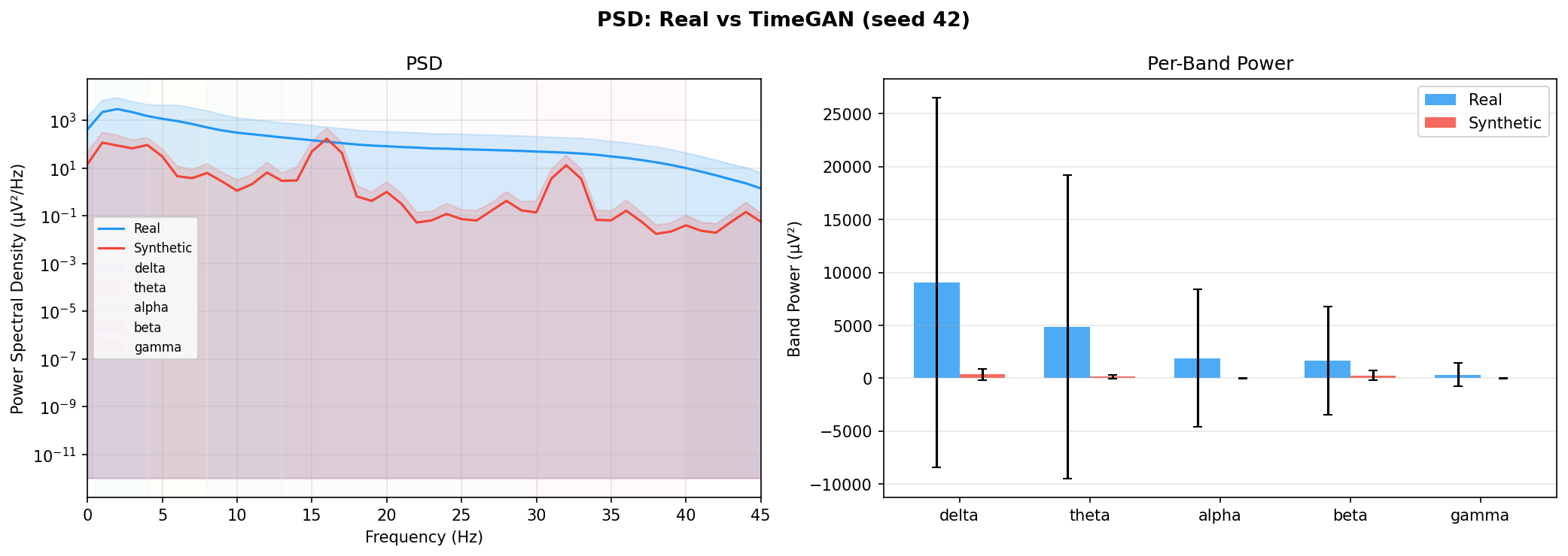
Seed 123
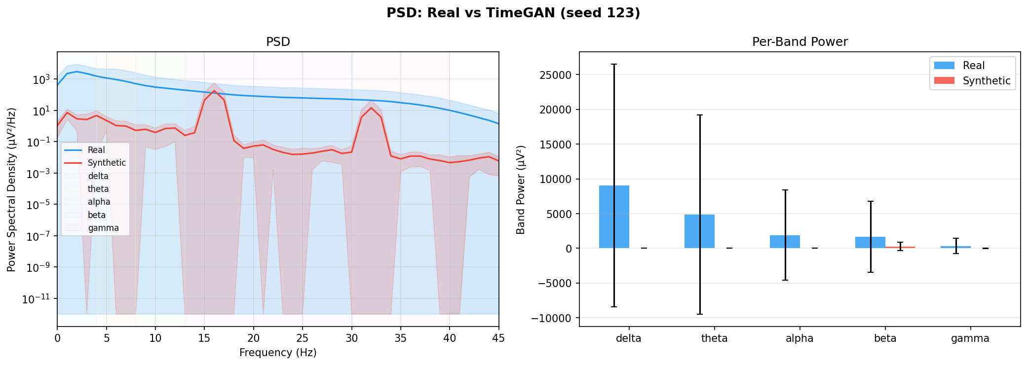
Seed 456
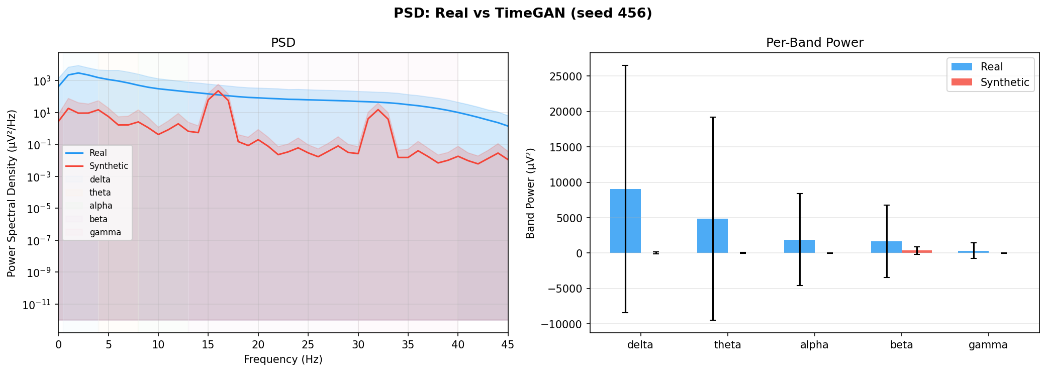
Autocorrelation - temporal dependence structure:
Seed 42
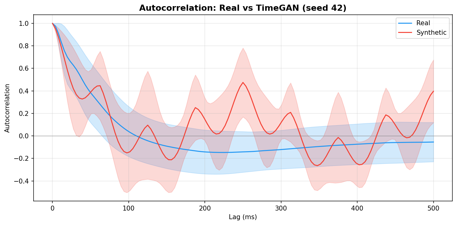
Seed 123
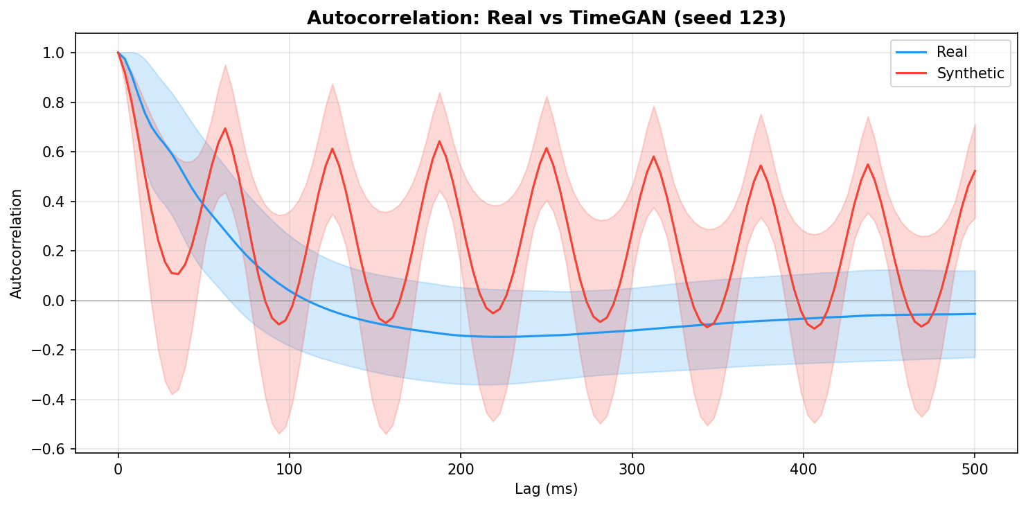
Seed 456
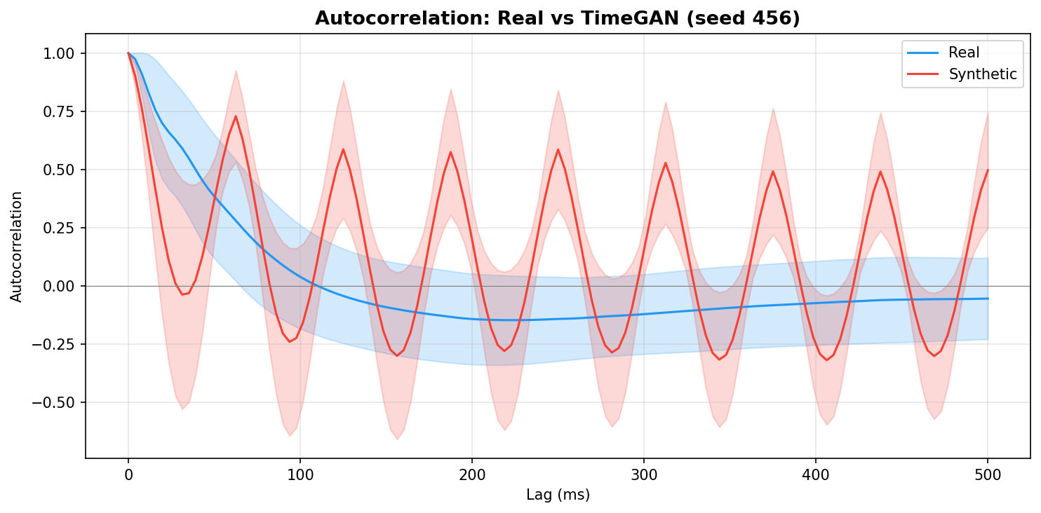
Per-channel amplitude distribution (mean and std):
Seed 42
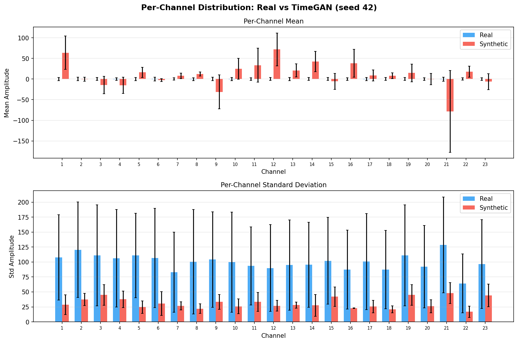
Seed 123
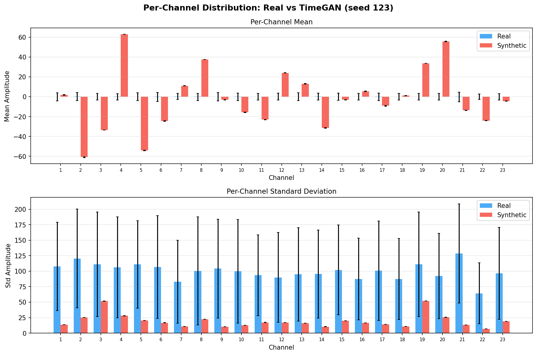
Seed 456
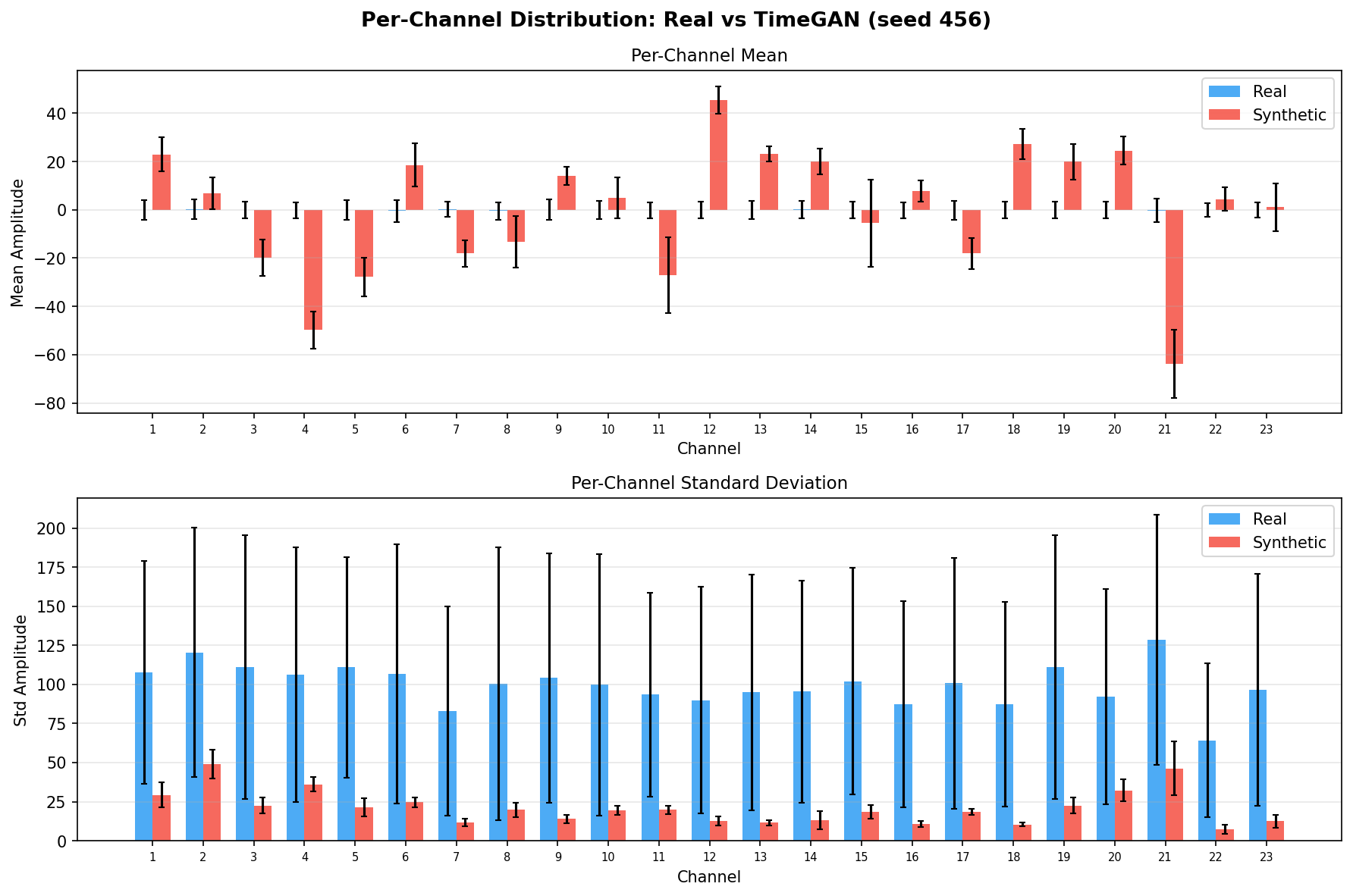
Waveform examples - real vs synthetic:
Seed 42
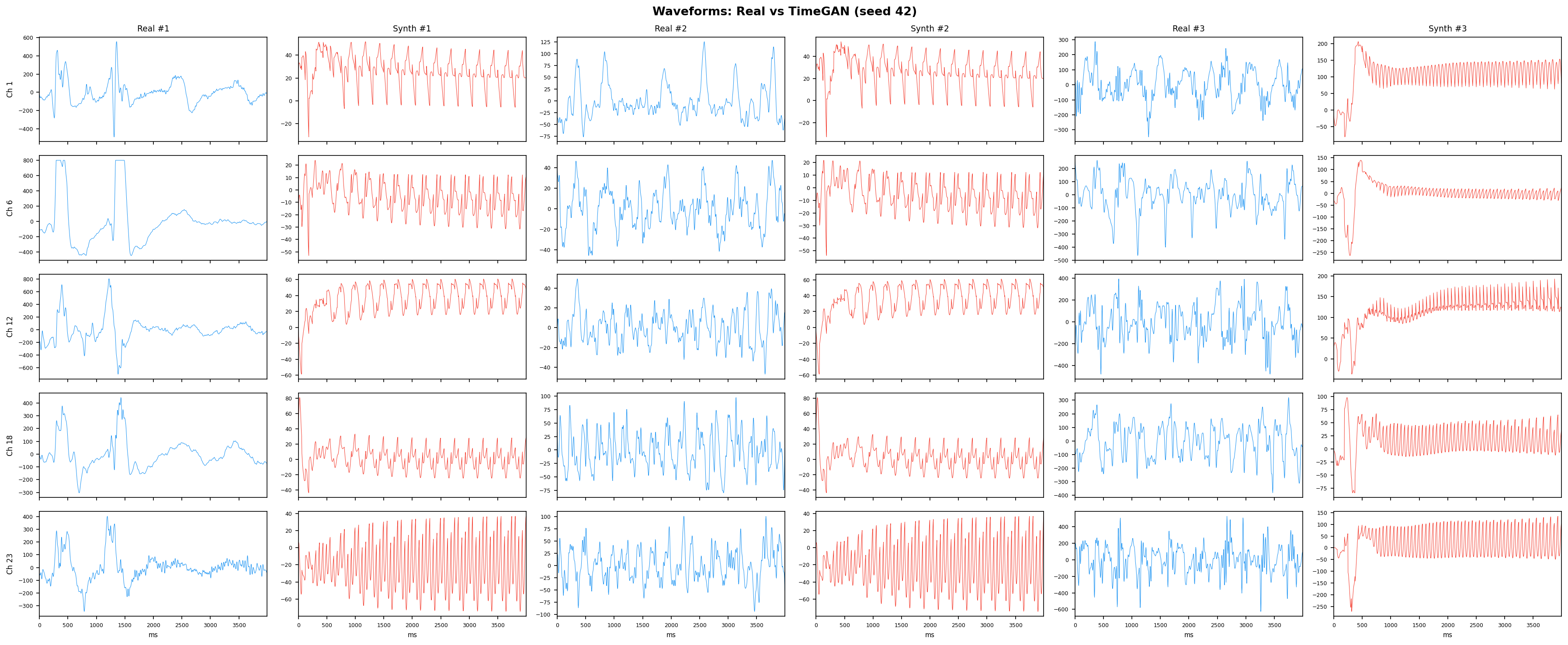
Seed 123
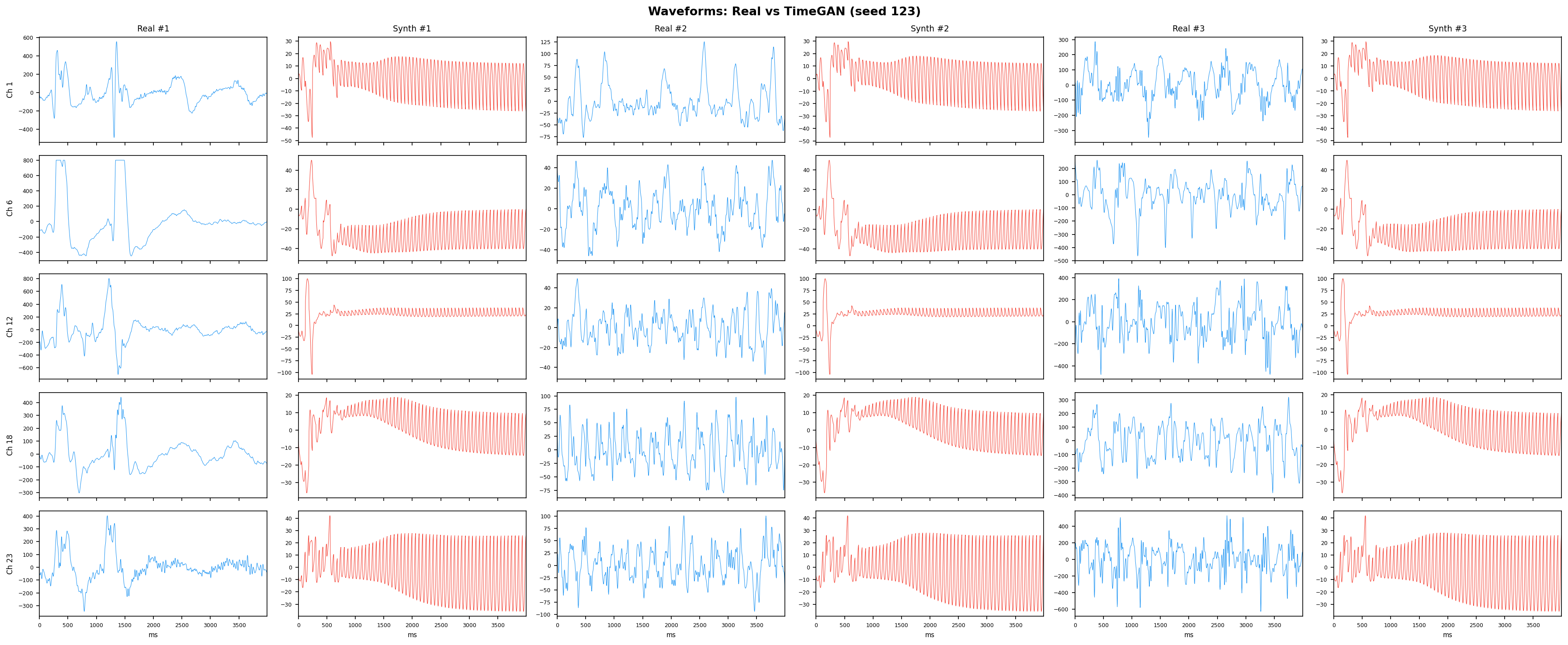
Seed 456
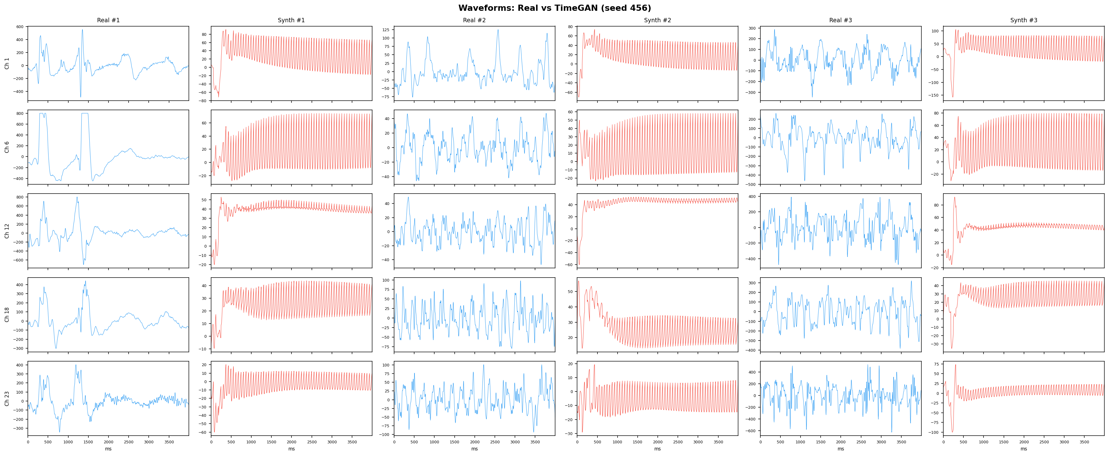
t-SNE embedding - do synthetic samples overlap with real?
Seed 42
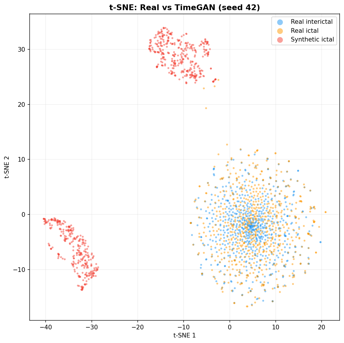
Seed 123
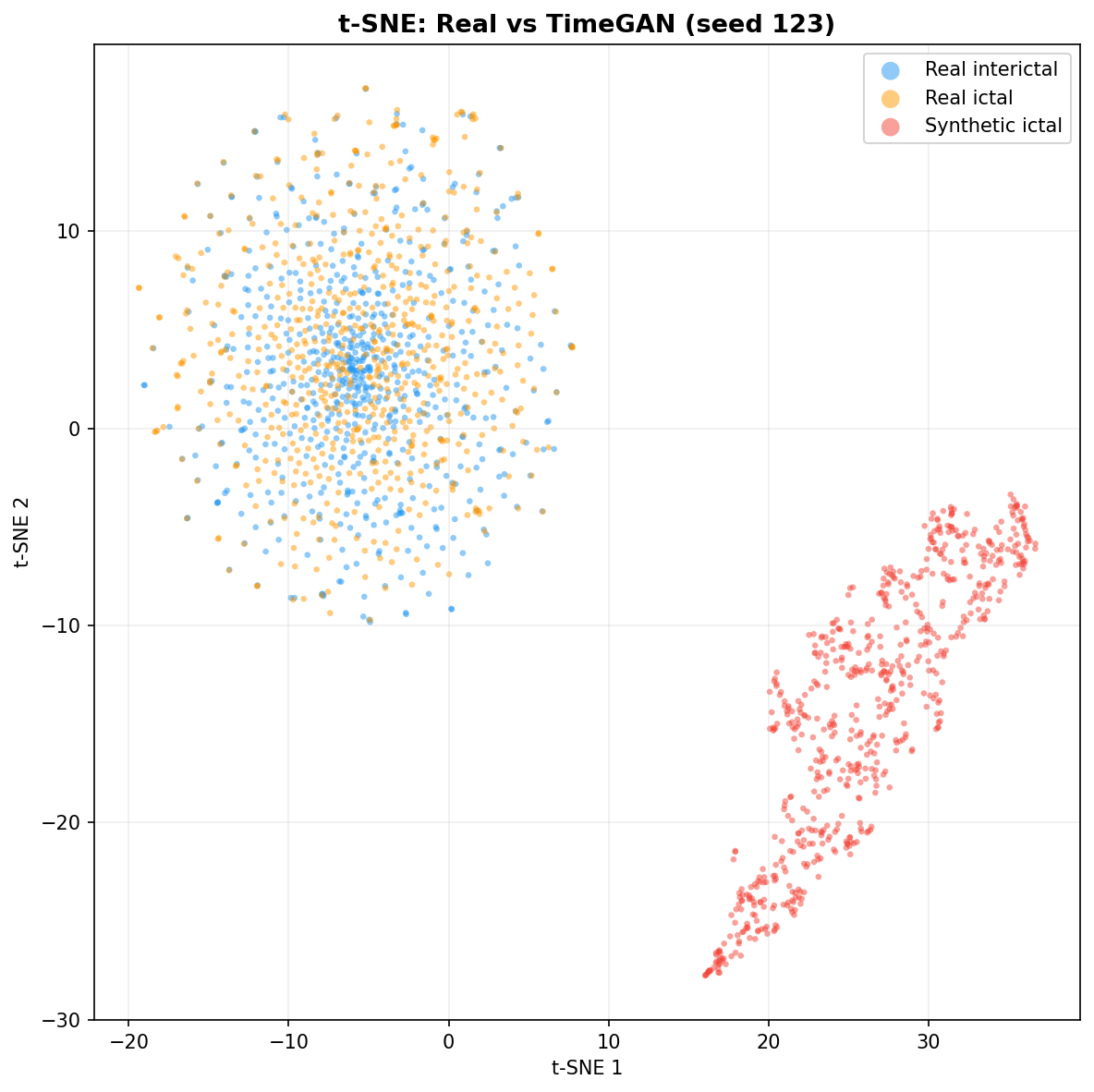
Seed 456
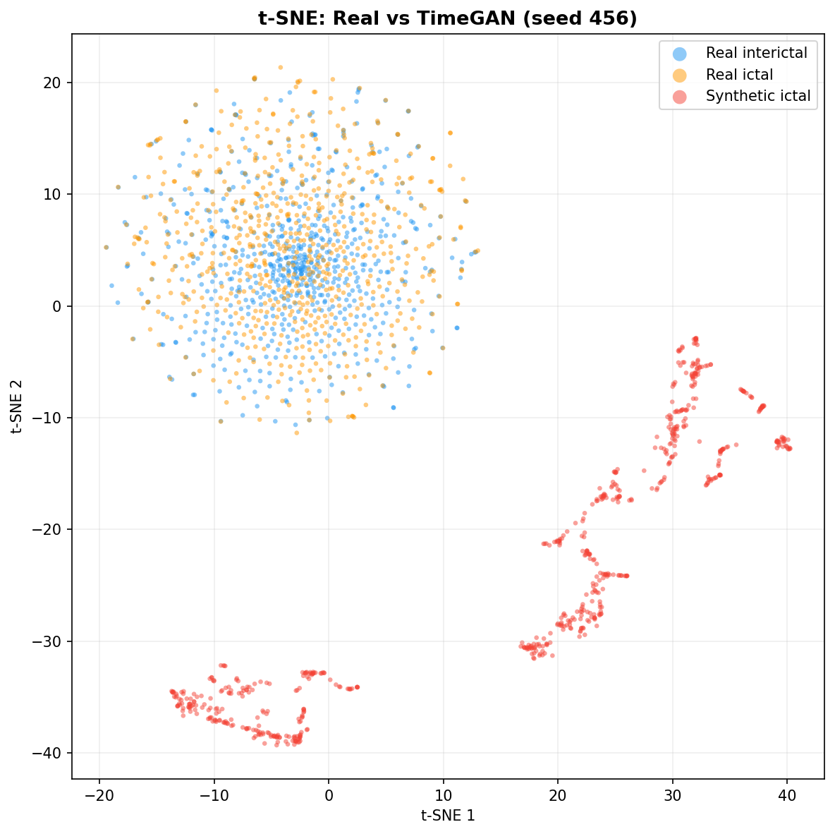
Fidelity plots - CVAE (E4) - all seeds
Power Spectral Density - real (blue) vs synthetic (red):
Seed 42
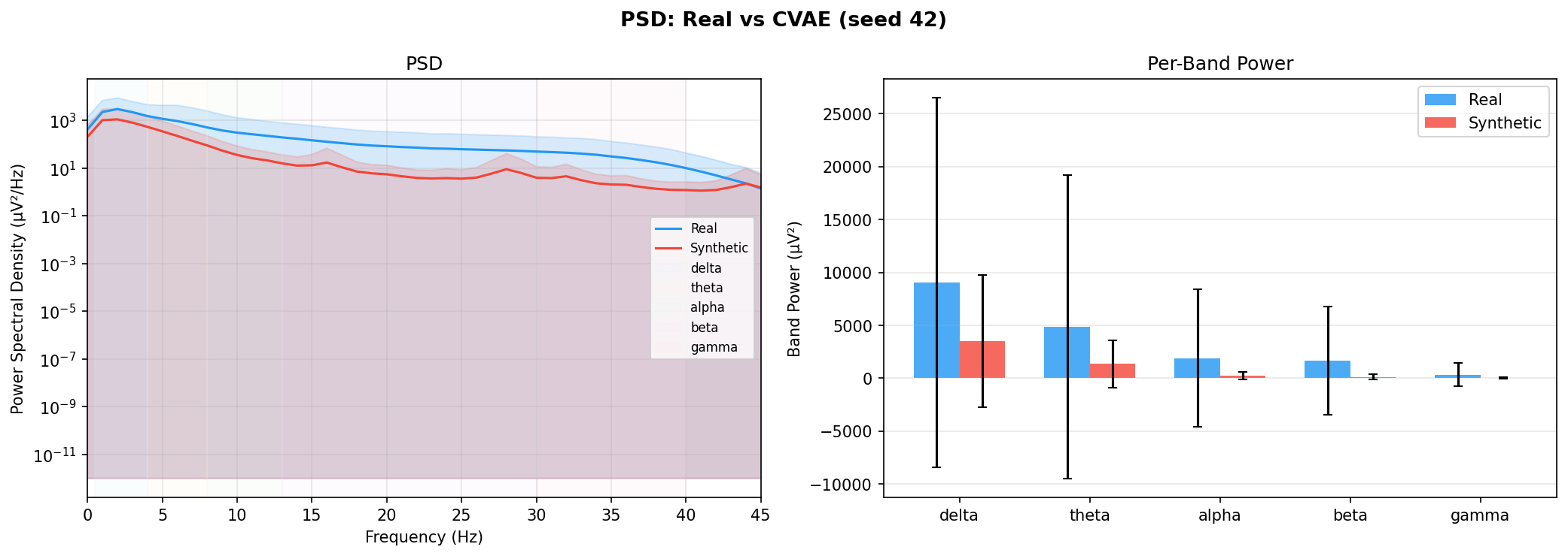
Seed 123

Seed 456

Autocorrelation - temporal dependence structure:
Seed 42
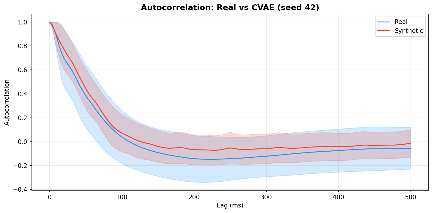
Seed 123

Seed 456
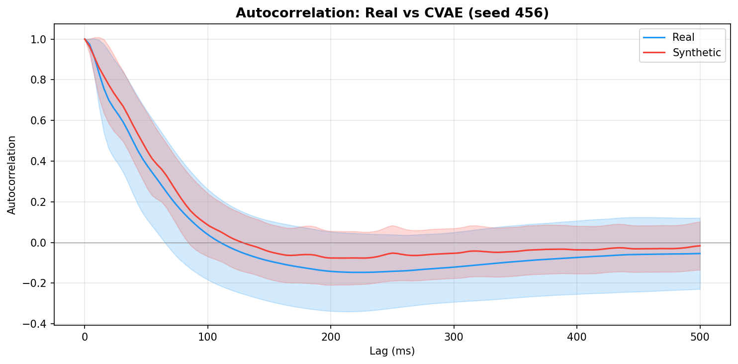
Per-channel amplitude distribution (mean and std):
Seed 42
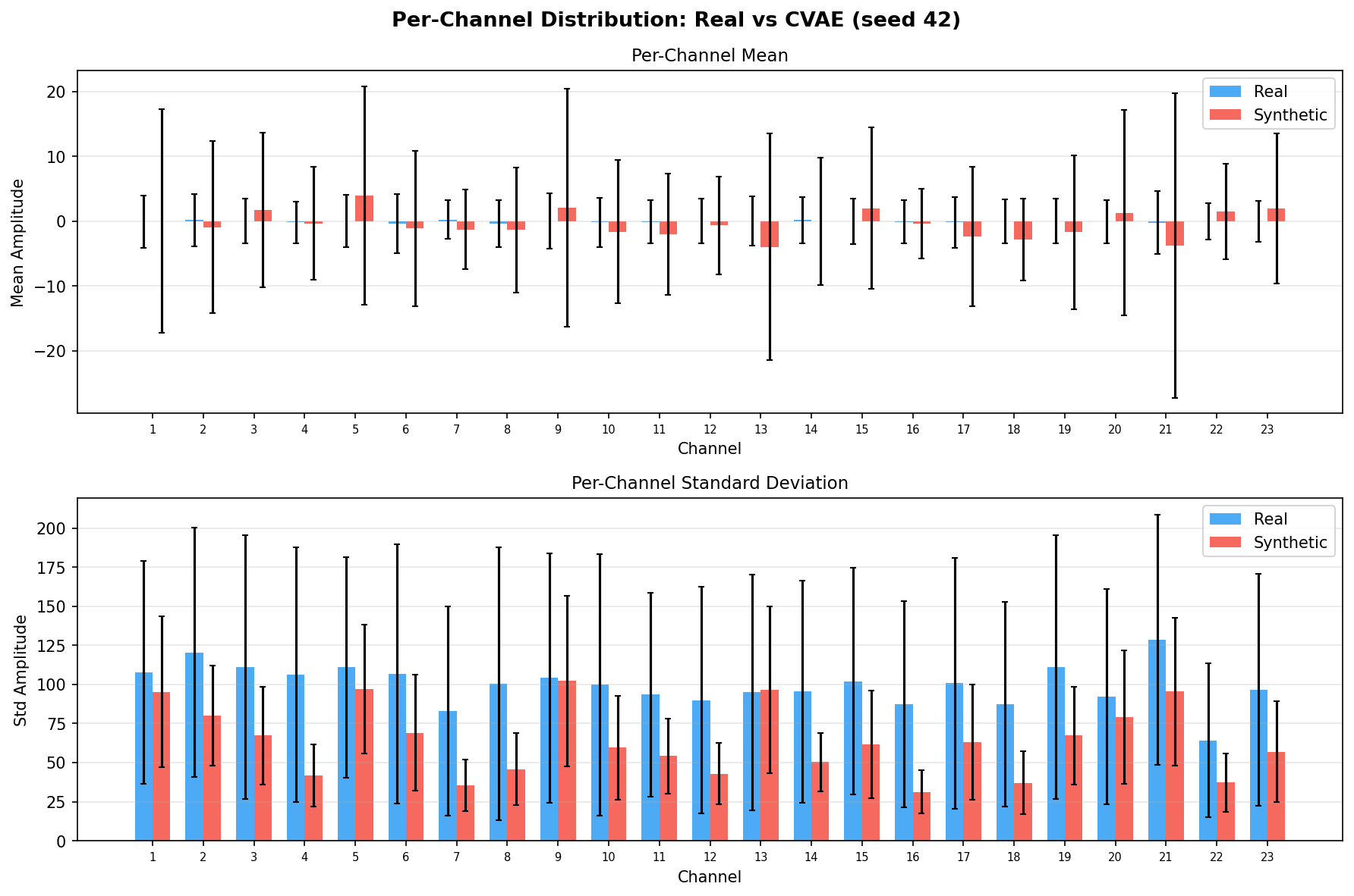
Seed 123
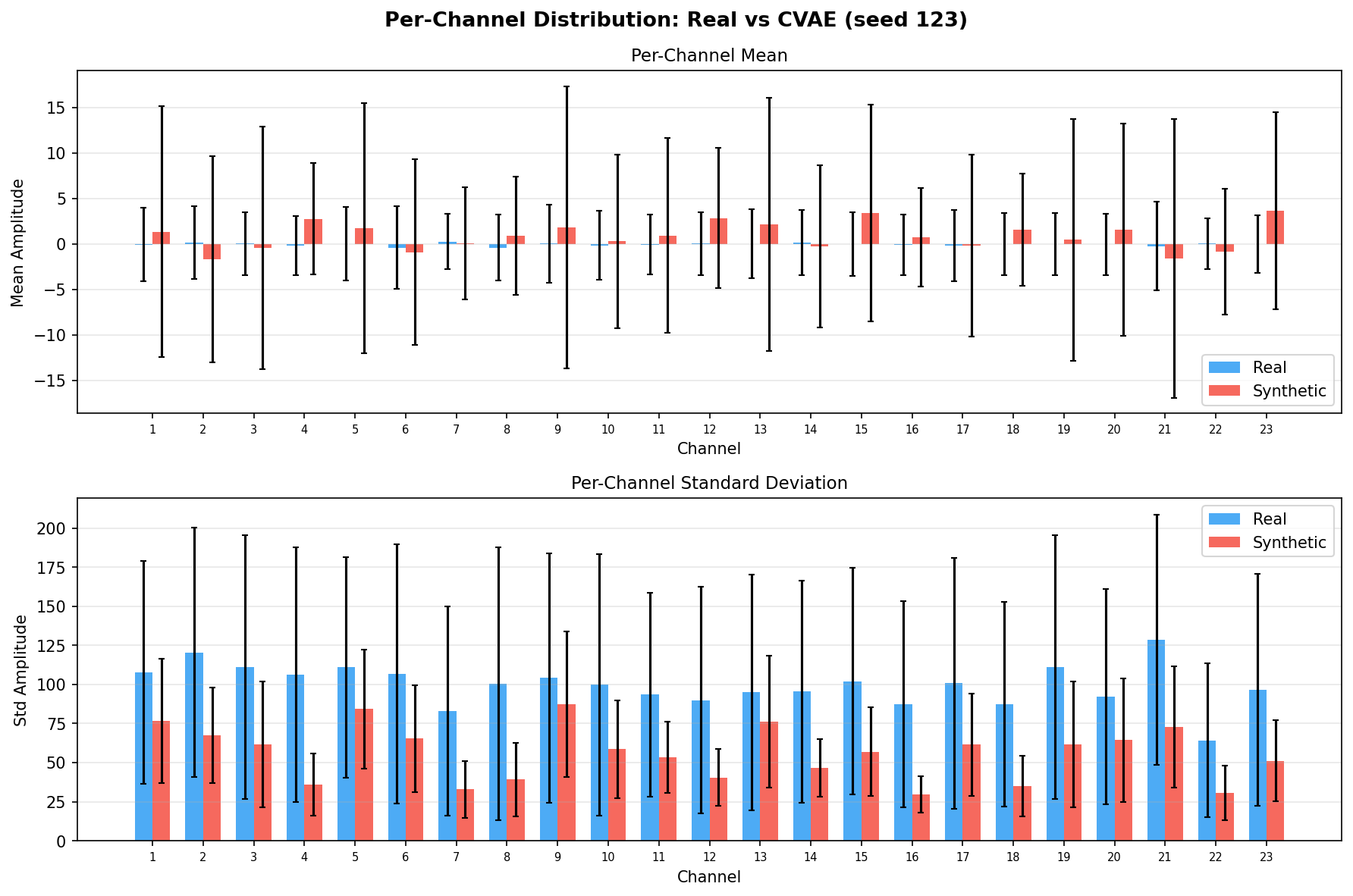
Seed 456
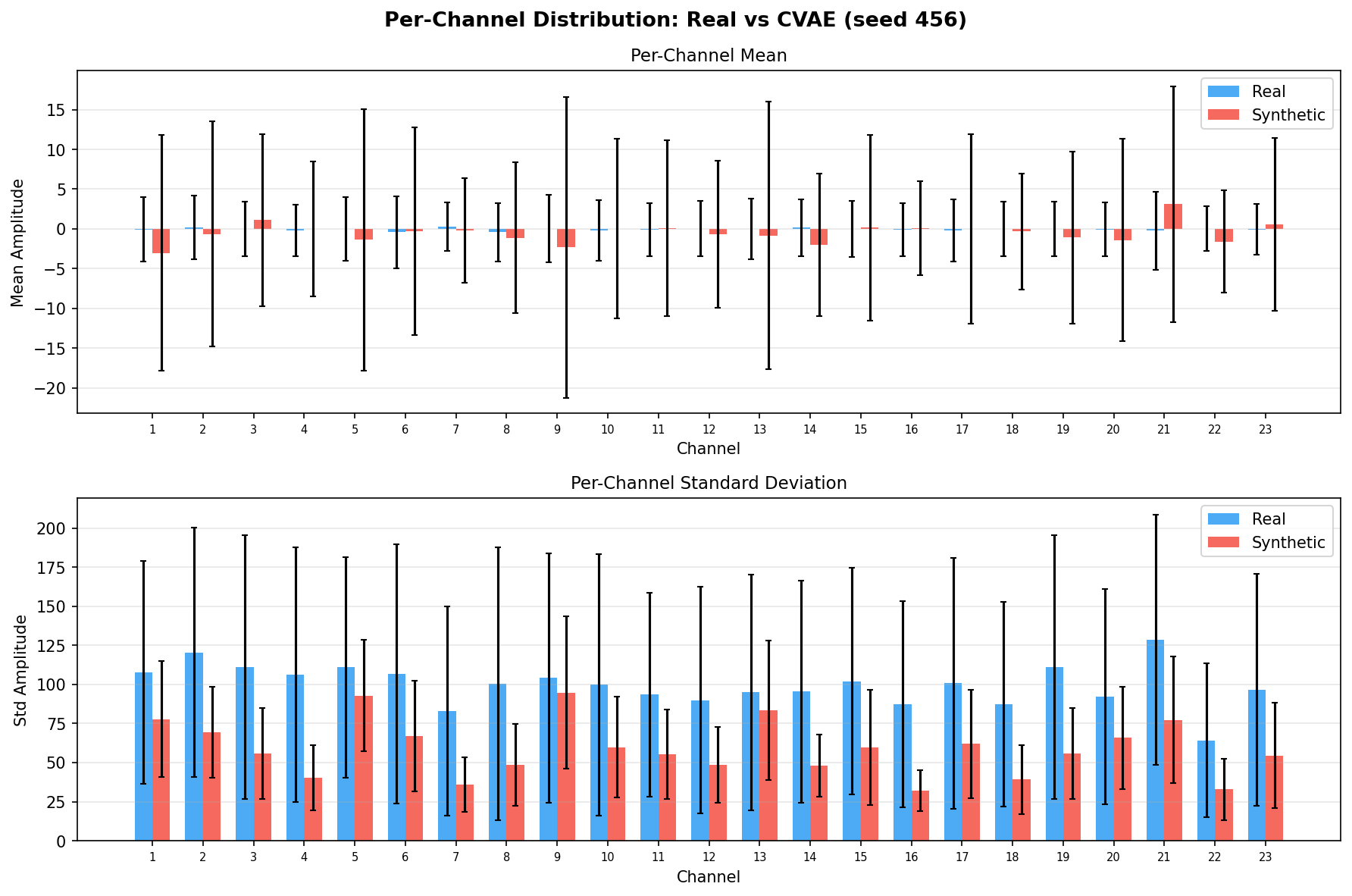
Waveform examples - real vs synthetic:
Seed 42
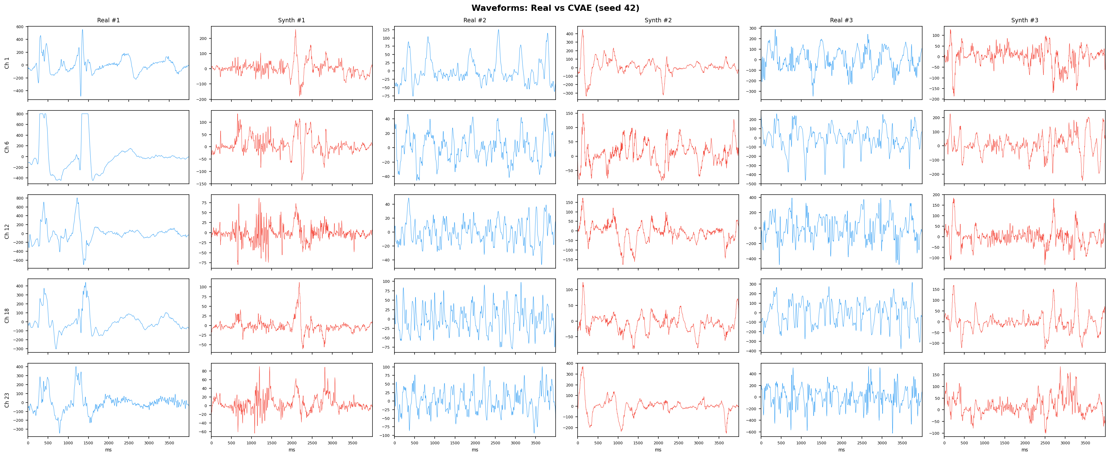
Seed 123
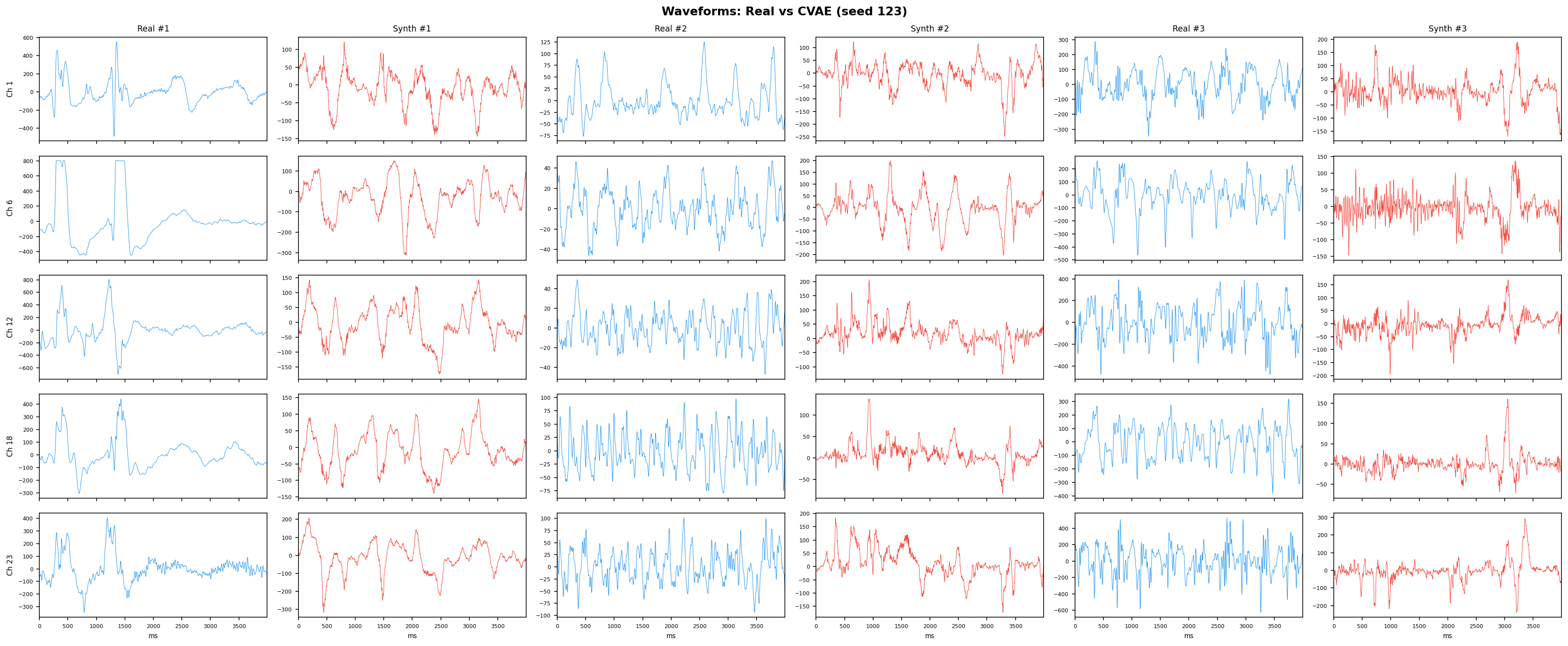
Seed 456
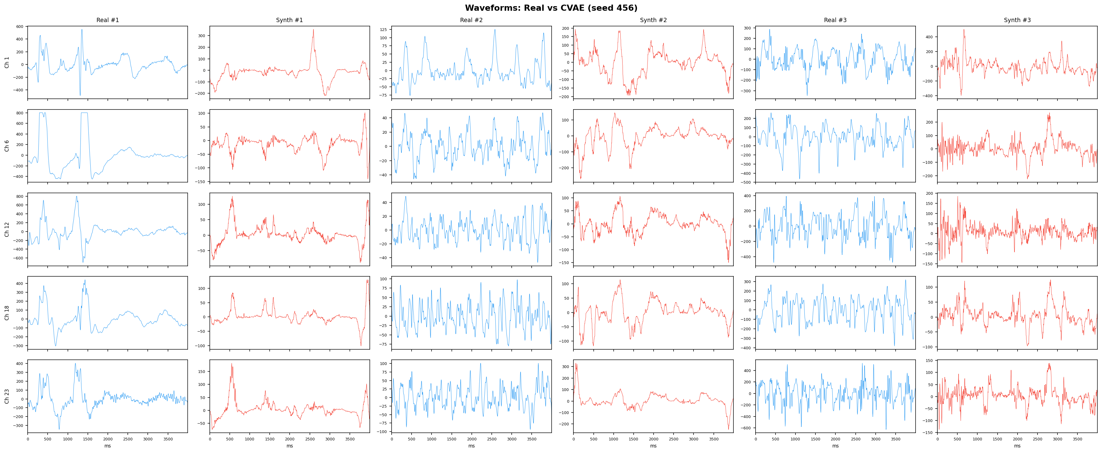
t-SNE embedding - do synthetic samples overlap with real?
Seed 42
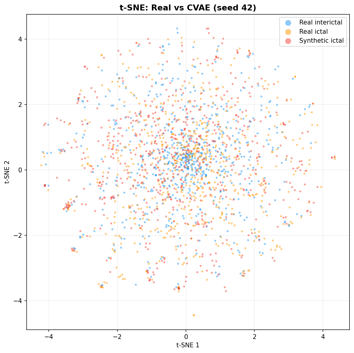
Seed 123
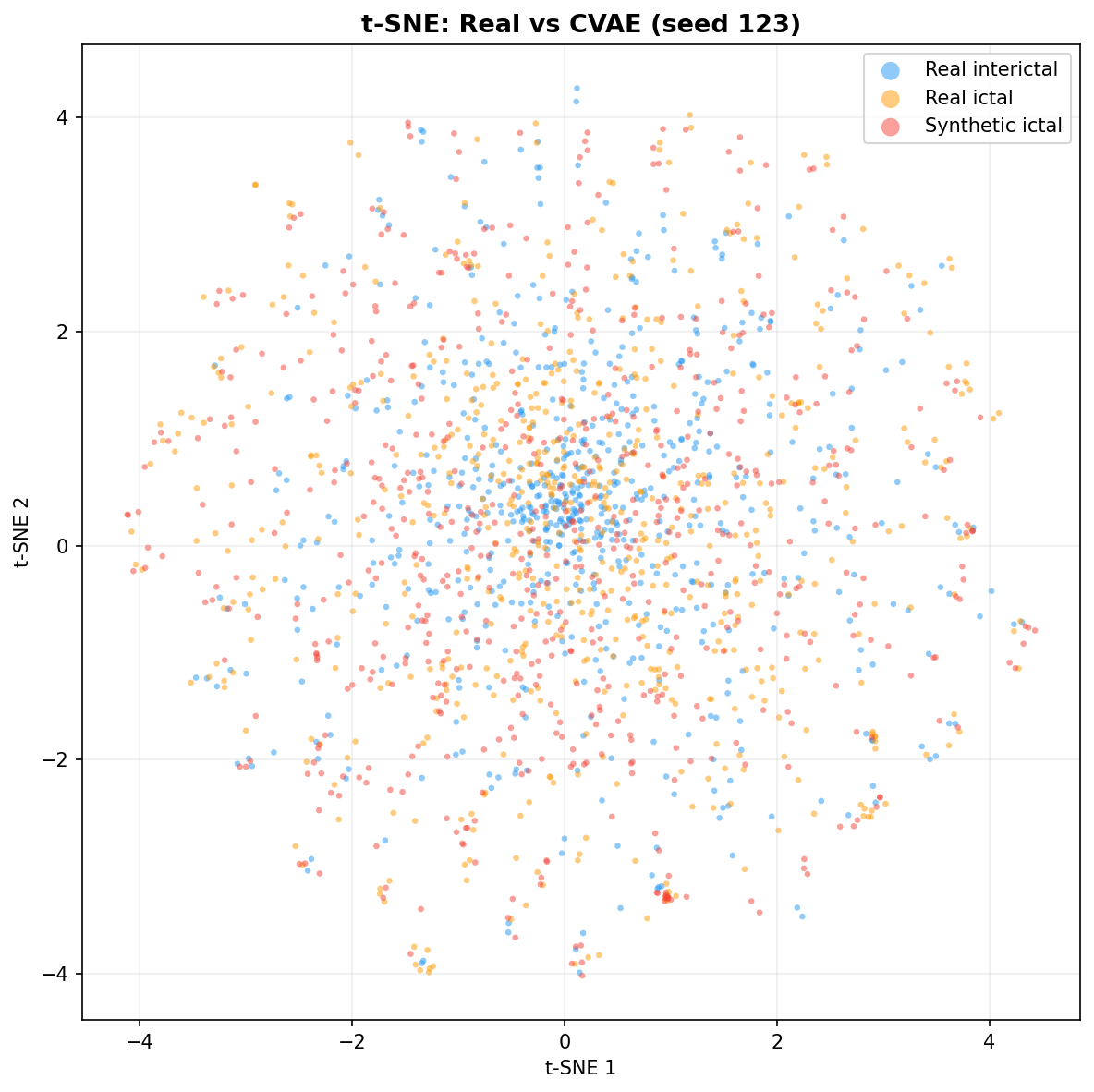
Seed 456
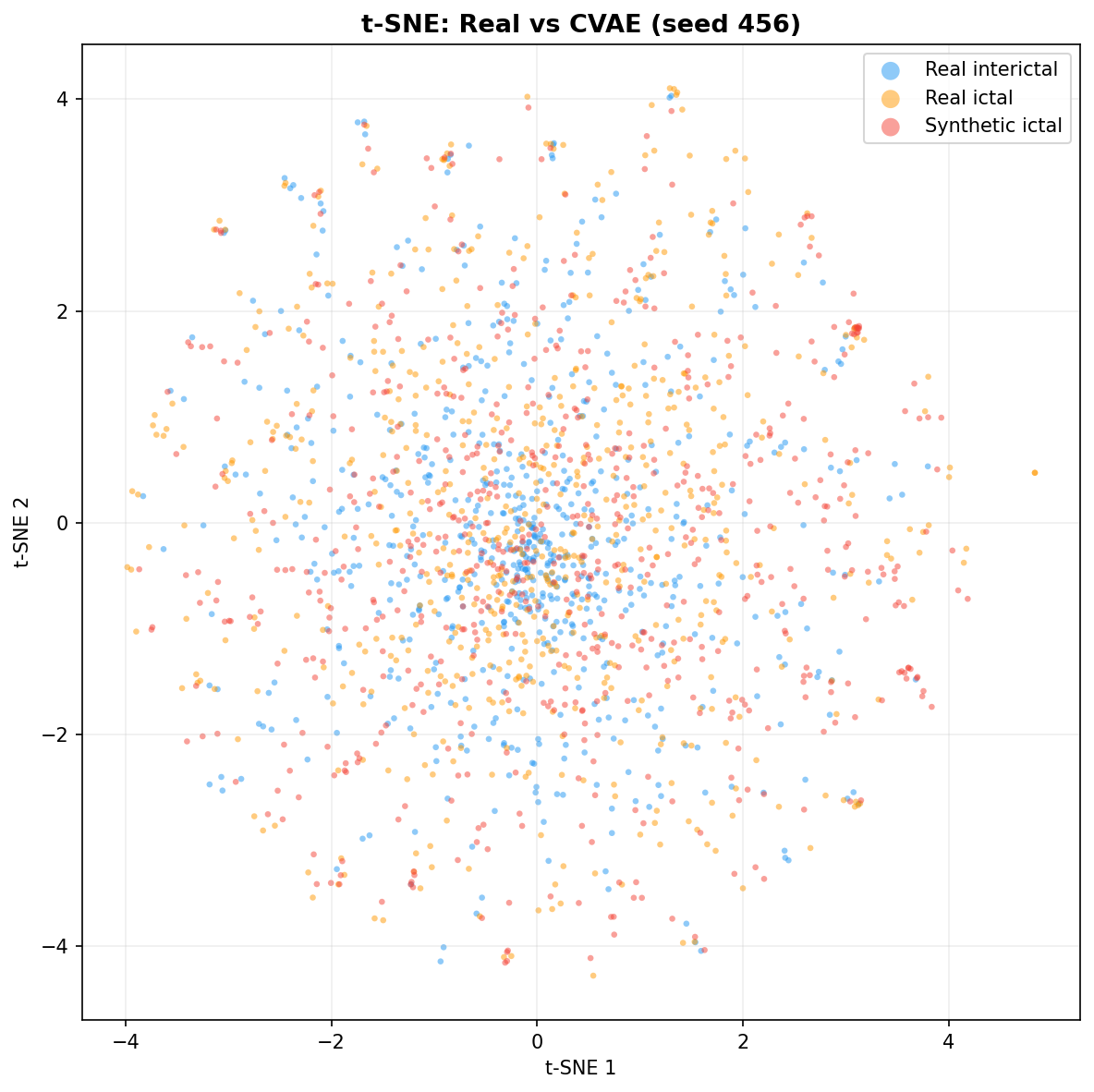
Fidelity plots - LDM (E5) - all seeds
Power Spectral Density - real (blue) vs synthetic (red):
Seed 42

Seed 123
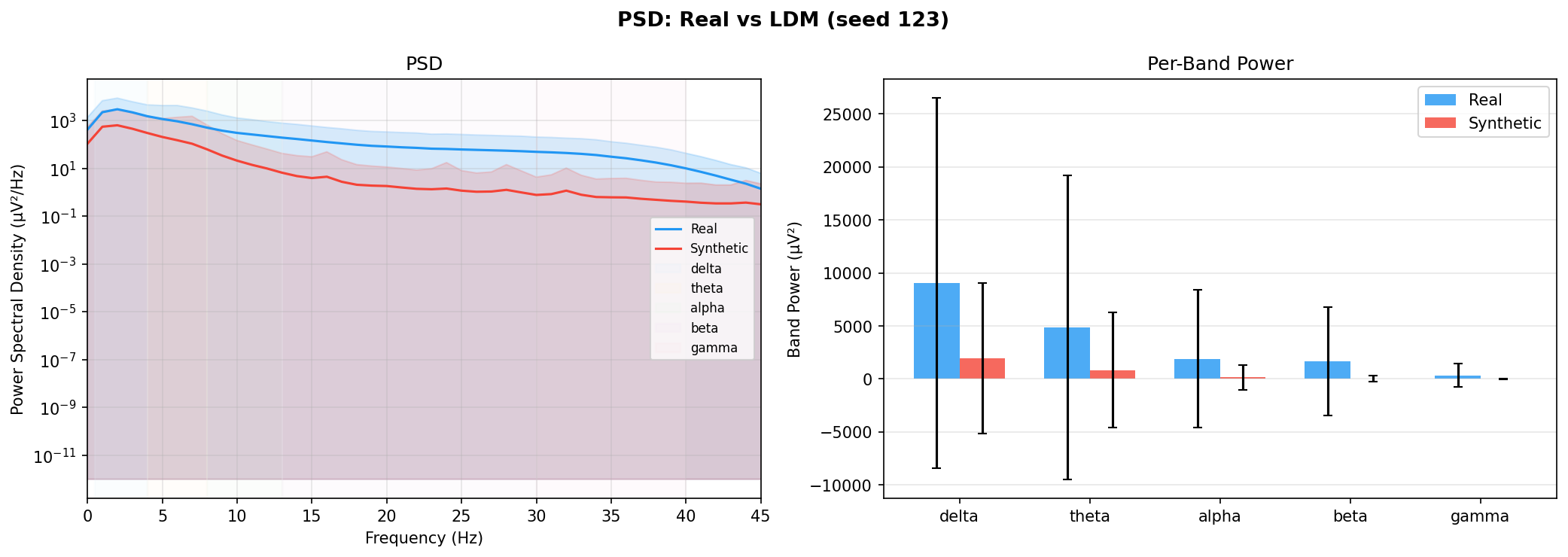
Seed 456

Autocorrelation - temporal dependence structure:
Seed 42
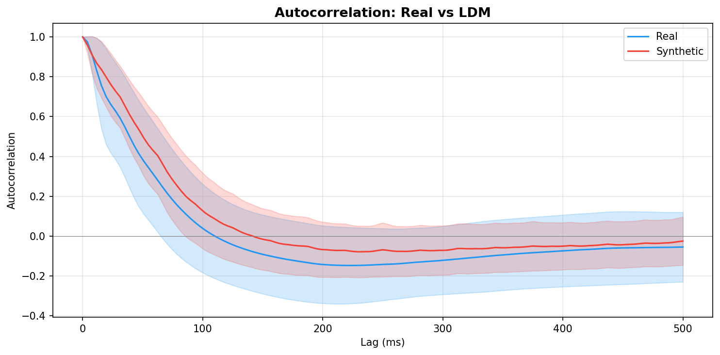
Seed 123
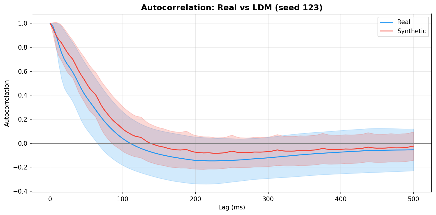
Seed 456
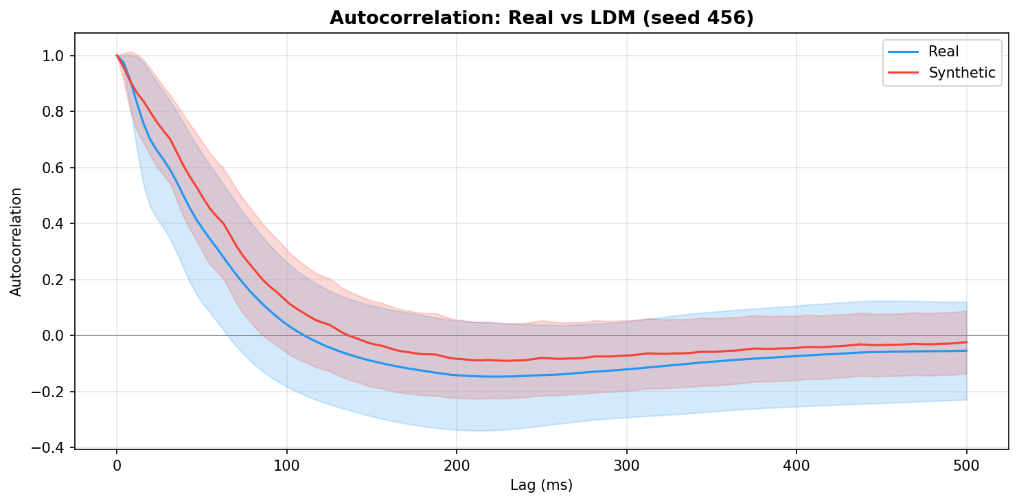
Per-channel amplitude distribution (mean and std):
Seed 42
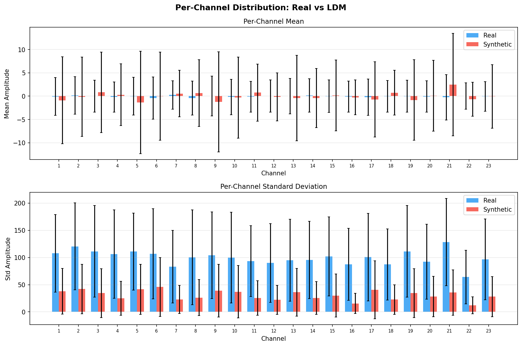
Seed 123
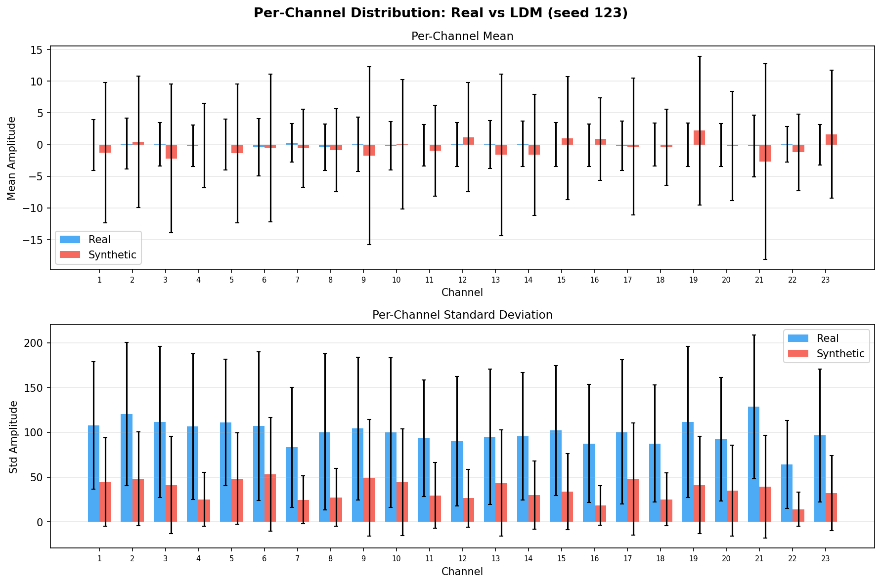
Seed 456
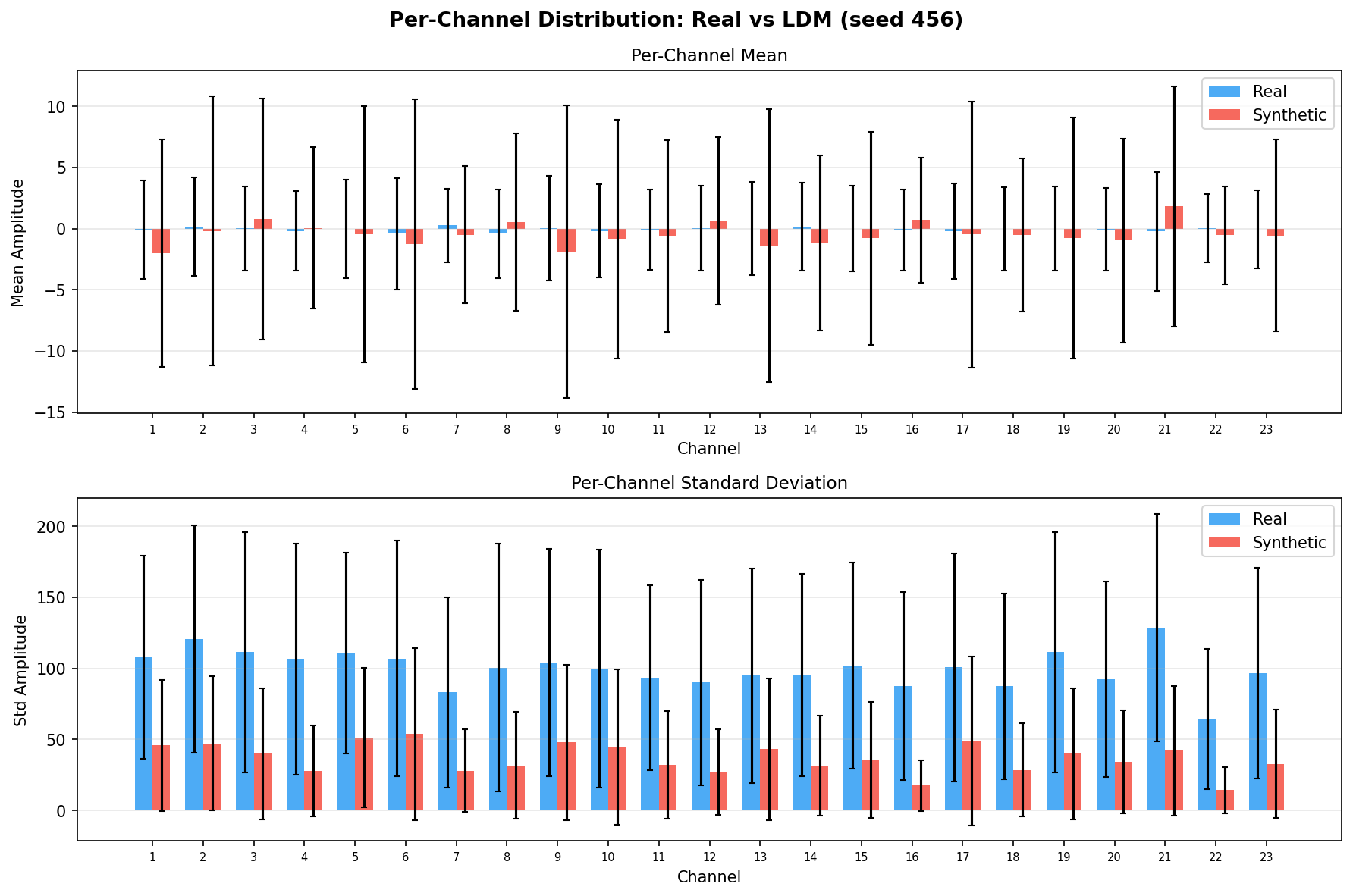
Waveform examples - real vs synthetic:
Seed 42
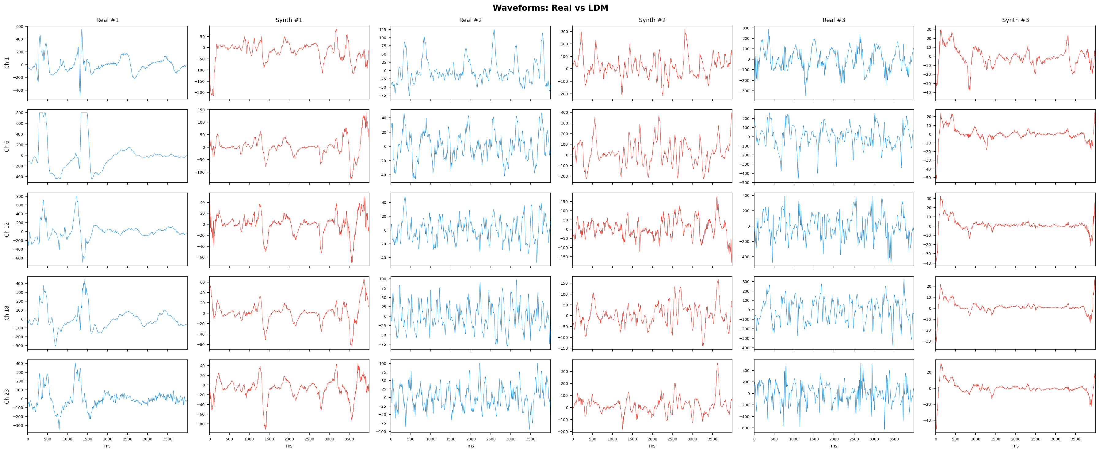
Seed 123
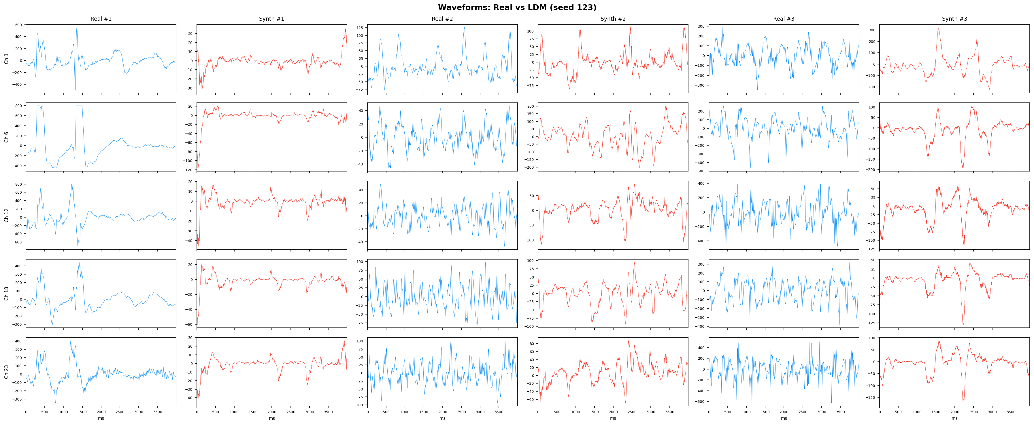
Seed 456
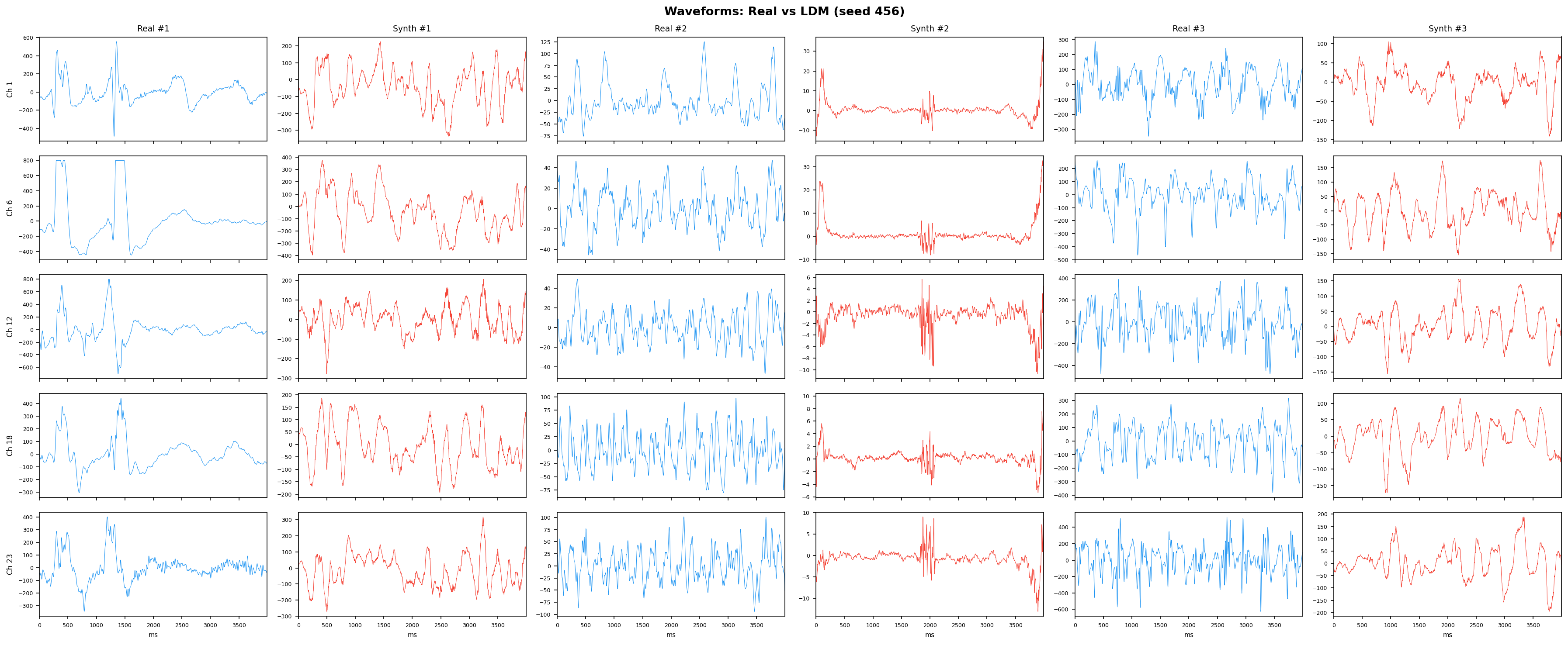
t-SNE embedding - do synthetic samples overlap with real?
Seed 42
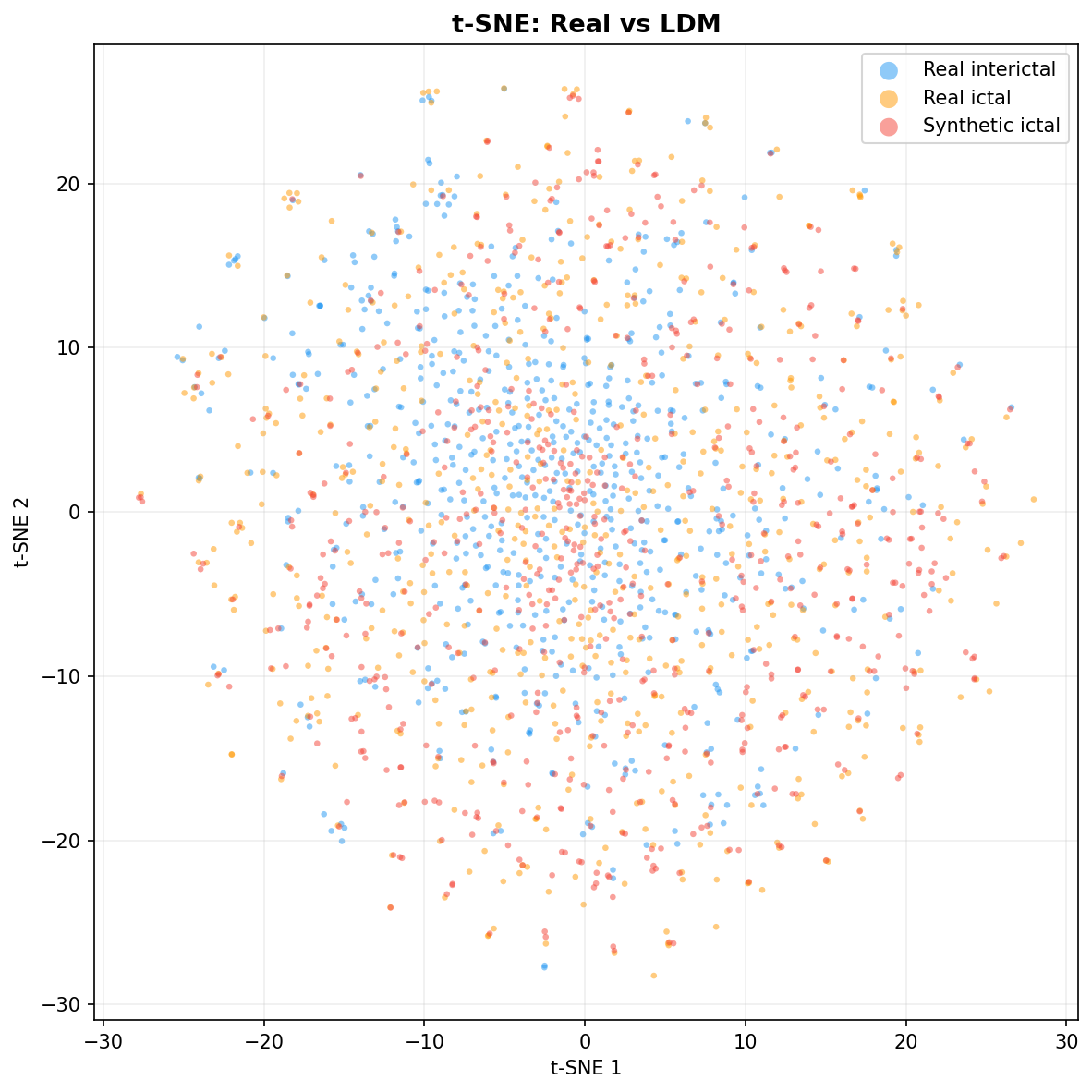
Seed 123
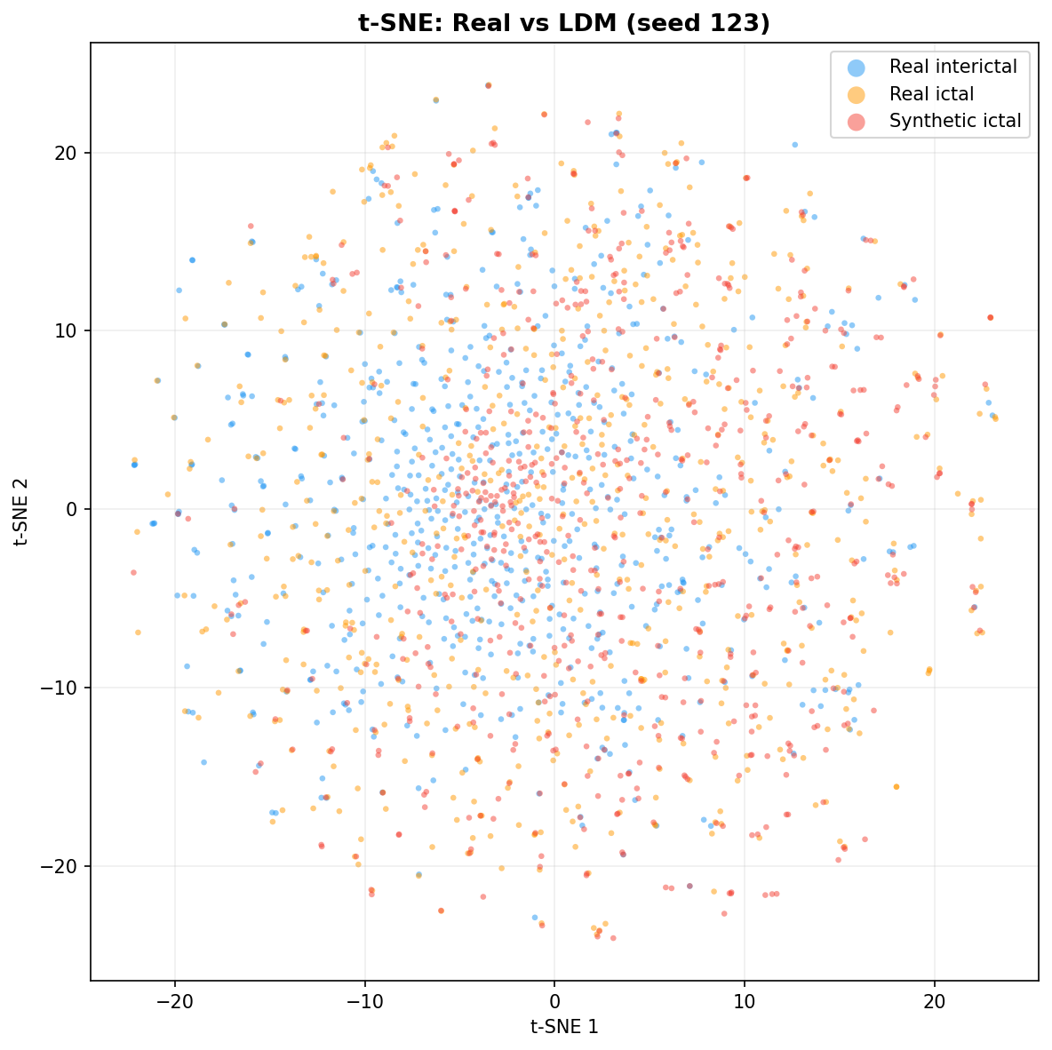
Seed 456
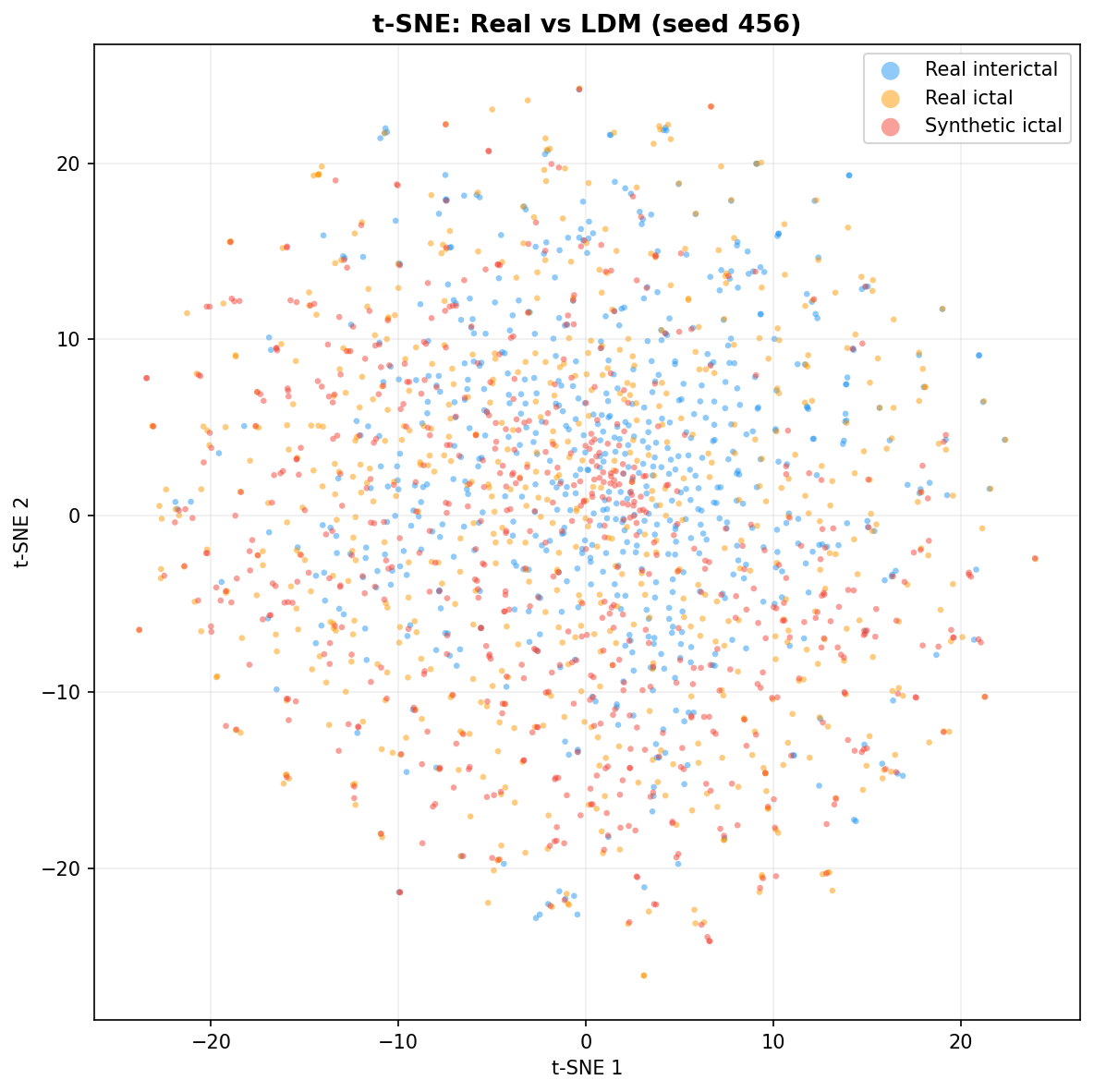
TimeGAN has a serious problem with high-frequency content. KL divergence above 2.0 in beta (13-30 Hz) and gamma (30-40 Hz) means it's producing signals with completely wrong spectral shape in those bands. The GRU architecture captures slow dynamics (delta/ theta are okay) but can't reproduce fast oscillations. This is visible in the waveforms too - they look smooth where real seizures have sharp transients.
CVAE has the best overall spectral match across all five bands (all KL < 0.05). It's also the hardest to distinguish from real data by accuracy (0.709 - closest to the ideal 0.5). The 1D-Conv architecture preserves frequency content at all scales because convolutions operate directly on the waveform.
LDM is best at low frequencies (delta/ theta) where most seizure energy lies, but slightly worse than CVAE in alpha. The iterative denoising process (50 DDIM steps) smooths some high-frequency detail. However, it has the lowest C2ST AUROC (0.680) meaning the classifier's confidence in its real-vs-synthetic predictions is lower - the mistakes it does make are less extreme.
Real ictal EEG has a smooth, monotonically decaying autocorrelation function - high at short lags (0-50 ms), crossing zero around 100 ms, and flattening near zero at longer lags. This reflects the continuous, oscillatory nature of brain signals.
TimeGAN produces signals with highly irregular autocorrelation: instead of smooth decay, the function oscillates wildly between positive and negative values at medium-to-long lags (100-500 ms), with very wide variance bands. This means the temporal structure is inconsistent across samples - some follow the real pattern, others are erratic. The GRU captures short-range dependencies (initial decay matches) but introduces spurious periodicities at longer timescales.
CVAE closely matches the real autocorrelation shape: smooth monotonic decay with the correct zero-crossing around 100 ms. The synthetic curve sits slightly above the real one at medium lags (100-300 ms), indicating marginally higher temporal smoothness (consistent with the VAE's tendency to produce slightly smoother outputs). Variance bands overlap substantially with the real data.
LDM shows nearly identical behaviour to the CVAE - expected since both use the same encoder/decoder. The autocorrelation decay is smooth and correctly shaped, with the synthetic curve again sitting slightly above real at medium lags. Both share the CVAE's latent space, so temporal structure is primarily determined by the decoder's ability to reconstruct smooth signals from compressed representations.
The 23×23 correlation matrix shows which EEG channels move together. For real ictal data, nearby electrodes are strongly correlated (seizures propagate spatially), creating a characteristic block-diagonal structure with off-diagonal correlations reflecting the propagation pattern.
TimeGAN partially preserves the spatial pattern (the overall structure of which channels correlate is visible) but the difference matrix shows systematic errors: correlation magnitudes are attenuated, meaning the generator produces channels that are less correlated than reality. This is consistent with mode collapse - if the generator produces more uniform outputs, inter-channel variation is reduced.
CVAE preserves spatial structure well. The correlation matrix visually resembles the real one, and the difference matrix shows small, relatively uniform residuals. The 1D convolutional architecture processes all 23 channels jointly, naturally learning inter-channel relationships during reconstruction.
LDM shows similar spatial preservation to the CVAE (same encoder/decoder). The difference matrix is comparable in magnitude and pattern, confirming that spatial structure is primarily encoded by the shared autoencoder rather than the generation method.
Each EEG channel has characteristic amplitude statistics (mean near zero after bandpass filtering, standard deviation ~85-130 uV for real ictal windows depending on the channel).
TimeGAN fails significantly on amplitude: per-channel means deviate from zero (offsets of 20-80 uV on several channels), and per-channel standard deviations are dramatically reduced (~25-45 uV vs real ~85-130 uV). The generator produces signals that are both offset and compressed in amplitude - about 3x lower variability than real seizures. This amplitude mismatch alone would make the synthetic data easy to detect by a downstream classifier.
CVAE preserves per-channel means well (all near zero) but shows reduced standard deviation compared to real data (~50-95 uV vs ~85-130 uV). This is the classic VAE smoothing effect: the KL regularisation encourages the decoder to produce outputs closer to the mean, reducing extreme amplitudes. Still much better than TimeGAN - the amplitude profile is recognisably correct even if somewhat compressed.
LDM has correct per-channel means (near zero) but shows the most severe amplitude reduction (~20-50 uV vs ~85-130 uV). The iterative denoising in latent space, combined with the CVAE decoder's smoothing tendency, produces signals with correct frequency content but lower dynamic range. This is the main weakness that the C2ST likely exploits to distinguish LDM outputs from real data.
These metrics answer different questions about synthetic quality. KL divergence asks "is the frequency content right?" Autocorrelation asks "is the temporal structure right?" Cross-channel correlation asks "are the spatial relationships right?" Per-channel distributions ask "are the amplitudes right?" C2ST asks "taking everything together, can anything tell them apart?"
No generator passes all tests perfectly, but the failure modes differ. TimeGAN fails at spectral, temporal, and amplitude levels - fundamental signal properties are wrong. CVAE passes spectral and temporal tests well but slightly compresses amplitudes (characteristic VAE smoothing). LDM has excellent spectral fidelity (especially low-frequency) and correct temporal structure, but compresses amplitudes more than CVAE.
These results explain the downstream utility pattern: TimeGAN's synthetic data is fundamentally wrong in multiple dimensions, so it can't help detection. CVAE and LDM both produce spectrally and temporally correct signals - the amplitude compression affects realism but still provides useful training signal for the frozen detector, because the frequency content and timing are correct.
Downstream Utility - All Experiments (single-split)
Does the synthetic data actually help seizure detection? Frozen detector trained with augmented data, tested on held-out patients.
What this table shows: The same frozen 49K-param 1D-CNN detector is trained under different data conditions and tested on the same 4 held-out patients. Any performance difference comes from the training data, not the model.
AUPRC is the primary metric - it only gives credit for correct, confident seizure predictions. Higher = better. With <0.4% seizure prevalence, even 0.20 represents meaningful detection ability.
Caveat: These are single-split results (one fixed train/test partition). They indicate trends but are NOT the final publishable numbers - those come from the full LOPO evaluation (23 folds × 3 seeds = 69 runs per experiment).
Mean ± std across 3 seeds (42, 123, 456). Single fixed split: 18 train/ 2 val/ 4 test patients. Training times are avg/ seed on RTX 3080 Ti (Gen. = generator, Det. = detector).
| Experiment | AUPRC | AUROC | F1 | Sens. @ 95% Spec. | Gen. | Det. |
|---|---|---|---|---|---|---|
| E1 Baseline (real only) | 0.177 ± 0.054 | 0.877 ± 0.036 | 0.287 ± 0.077 | 0.618 ± 0.097 | — | ~205 min |
| E2 SMOTE | 0.069 ± 0.062 | 0.546 ± 0.136 | 0.167 ± 0.115 | 0.300 ± 0.182 | — | ~90 min |
| E2 ADASYN | 0.108 ± 0.073 | 0.556 ± 0.034 | 0.233 ± 0.151 | 0.307 ± 0.091 | — | ~79 min |
| E3 TimeGAN | 0.174 ± 0.084 | 0.703 ± 0.134 | 0.261 ± 0.084 | 0.481 ± 0.122 | ~17 min | ~84 min |
| E4 CVAE | 0.175 ± 0.073 | 0.844 ± 0.074 | 0.263 ± 0.103 | 0.602 ± 0.207 | ~42 min | ~99 min |
| E5 LDM | 0.227 ± 0.019 | 0.893 ± 0.013 | 0.367 ± 0.020 | 0.717 ± 0.077 | ~58 min | ~72 min |
E1 baseline (real data + class-weighted loss) achieves AUPRC 0.177 - this is the bar everything else must beat. Note the high variance across seeds, typical for small test sets.
SMOTE and ADASYN (E2) actively hurt performance - SMOTE drops AUPRC to 0.069. This confirms the thesis motivation: naive interpolation in 23,552-dimensional space destroys temporal and spectral structure. The synthetic windows are just blends that confuse the detector rather than teaching it new patterns.
TimeGAN (E3) matches the baseline (0.174 vs 0.177) but doesn't improve it. Combined with the fidelity results above (wrong spectral shape, erratic temporal structure), this makes sense: the synthetic data is different enough from real to not actively hurt, but too unrealistic to provide useful new signal.
CVAE (E4) also matches baseline (0.175) but with better AUROC. The good spectral fidelity translates to "doesn't hurt", but doesn't clearly help either at this ratio. High seed variance suggests the effect is inconsistent.
LDM (E5) is the only generator that clearly improves over baseline: +0.050 AUPRC (+29%), +0.080 F1 (+28%), +0.099 Sensitivity (+16%). Crucially, it also has the lowest variance across seeds, meaning the improvement is consistent. This aligns with its fidelity profile: best low-frequency reproduction (where seizure energy lives) combined with correct temporal structure.
Important: These are preliminary single-split results. The full LOPO evaluation will provide the statistically rigorous comparison across all 23 patients.
Per-experiment details (per-seed breakdowns, training epochs, timing - click to expand)
Baseline Results - 1D-CNN Detector (single-split, no augmentation)
Completed 26 Apr 2026 - 3 seeds, class-weighted cross-entropy loss, early stopping on validation AUPRC
| Metric | Seed 42 | Seed 123 | Seed 456 | Mean ± Std |
|---|---|---|---|---|
| AUPRC | 0.1047 | 0.1896 | 0.2355 | 0.1766 ± 0.0542 |
| AUROC | 0.8267 | 0.8978 | 0.9057 | 0.8767 ± 0.0355 |
| F1 | 0.1794 | 0.3281 | 0.3536 | 0.2870 ± 0.0768 |
| Sens. @ 95% Spec. | 0.4829 | 0.6639 | 0.7064 | 0.6177 ± 0.0969 |
| Per-patient AUPRC | 0.1366 | 0.2567 | 0.2857 | 0.2264 ± 0.0646 |
Non-Synthetic Control Results (single-split)
Completed 27 Apr 2026 - SMOTE and ADASYN, 3 seeds each, class-weighted cross-entropy loss, early stopping on validation AUPRC
E2 - SMOTE (k=5)
| Metric | Seed 42 | Seed 123 | Seed 456 | Mean ± Std |
|---|---|---|---|---|
| AUPRC | 0.1519 | 0.0047 | 0.0490 | 0.0685 ± 0.0617 |
| AUROC | 0.6633 | 0.3558 | 0.6187 | 0.5459 ± 0.1357 |
| F1 | 0.3118 | 0.0307 | 0.1589 | 0.1671 ± 0.1149 |
| Sens. @ 95% Spec. | 0.4938 | 0.0562 | 0.3498 | 0.2999 ± 0.1821 |
| Per-patient AUPRC | 0.1831 | 0.0063 | 0.0868 | 0.0921 ± 0.0723 |
E2 - ADASYN
| Metric | Seed 42 | Seed 123 | Seed 456 | Mean ± Std |
|---|---|---|---|---|
| AUPRC | 0.1822 | 0.0082 | 0.1329 | 0.1078 ± 0.0732 |
| AUROC | 0.5656 | 0.5916 | 0.5103 | 0.5558 ± 0.0339 |
| F1 | 0.3873 | 0.0280 | 0.2829 | 0.2327 ± 0.1509 |
| Sens. @ 95% Spec. | 0.3992 | 0.1824 | 0.3388 | 0.3068 ± 0.0913 |
| Per-patient AUPRC | 0.2258 | 0.0545 | 0.1104 | 0.1302 ± 0.0713 |
Both SMOTE and ADASYN underperform the E1 baseline across all metrics. Mean AUPRC drops from 0.1766 (E1) to 0.0685 (SMOTE) and 0.1078 (ADASYN).
Why do these methods hurt? SMOTE and ADASYN are tabular oversampling methods - they create new samples by interpolating between existing ones in feature space. EEG windows are 23 channels × 1,024 time steps (23,552 dimensions). In this high-dimensional space:
- Temporal coherence is destroyed. The 1D-CNN detector learns local temporal patterns via convolution. Interpolated signals mix the timing of features from two different windows, producing waveforms that look nothing like real seizures - sharp spikes and rhythmic discharges get averaged out.
- Curse of dimensionality. In 23K-dimensional space, k-nearest neighbors (k=5 for SMOTE) may not be meaningfully similar. The interpolation path between them passes through regions that don’t correspond to real EEG.
- E1 already handles imbalance. The class-weighted cross-entropy loss upweights seizure samples in the gradient. Adding low-quality synthetic samples on top dilutes the real signal rather than reinforcing it.
- Seed instability confirms the problem. SMOTE seed 123 collapses to AUPRC 0.0047 - near-chance. A single bad set of synthetic neighbors can derail the entire training run. Validation AUPRC trajectories oscillate epoch-to-epoch, unlike the smoother E1 curves.
This is exactly why the thesis tests generative models - TimeGAN, CVAE, and LDM can learn the temporal structure of ictal EEG and produce windows that preserve spectral and morphological characteristics, rather than blending signals in flat feature space. The bar for generative models (E3–E5) remains the E1 baseline, not these controls.
TimeGAN Results - Synthetic Augmentation (single-split, ratio 1.0)
Completed 27 Apr 2026 - 3 seeds, TimeGAN-generated ictal windows (600 epochs × 3 phases), class-weighted cross-entropy loss, early stopping on validation AUPRC
| Metric | Seed 42 | Seed 123 | Seed 456 | Mean ± Std |
|---|---|---|---|---|
| AUPRC | 0.1370 | 0.0948 | 0.2907 | 0.1742 ± 0.0842 |
| AUROC | 0.8336 | 0.5191 | 0.7565 | 0.7031 ± 0.1338 |
| F1 | 0.1986 | 0.2051 | 0.3799 | 0.2612 ± 0.0840 |
| Sens. @ 95% Spec. | 0.5432 | 0.3114 | 0.5898 | 0.4815 ± 0.1218 |
| Per-patient AUPRC | 0.1360 | 0.1035 | 0.3434 | 0.1943 ± 0.1063 |
TimeGAN augmentation at 100% ratio produces results comparable to E1 baseline (mean AUPRC 0.1742 vs 0.1766). Unlike SMOTE/ADASYN (E2), the synthetic windows are realistic enough that adding them to training doesn't degrade things - but it doesn't clearly help either.
High seed variance is notable. Seed 456 hits AUPRC 0.2907 (higher than any E1 seed), while seed 123 drops to 0.0948. TimeGAN's 3-phase adversarial training is sensitive to initialisation - some seeds produce much better synthetic data than others. This is a known instability issue with GANs.
Key takeaway: generative augmentation preserves baseline performance (unlike tabular oversampling which actively hurts), but TimeGAN alone doesn't improve it. CVAE (E4) and LDM (E5) test whether different generation strategies can do better.
CVAE Results - Synthetic Augmentation (single-split, ratio 1.0)
Completed 29 Apr 2026 - 3 seeds, CVAE-generated ictal windows (LR warmup 5e-5 to 5e-4, log_var clamping, grad clip 1.0), class-weighted cross-entropy loss, early stopping on validation AUPRC
| Metric | Seed 42 | Seed 123 | Seed 456 | Mean ± Std |
|---|---|---|---|---|
| AUPRC | 0.2385 | 0.2141 | 0.0724 | 0.1750 ± 0.0732 |
| AUROC | 0.9082 | 0.8836 | 0.7396 | 0.8438 ± 0.0744 |
| F1 | 0.3294 | 0.3419 | 0.1170 | 0.2628 ± 0.1032 |
| Sens. @ 95% Spec. | 0.7462 | 0.7503 | 0.3086 | 0.6017 ± 0.2073 |
| Per-patient AUPRC | 0.3883 | 0.3616 | 0.1131 | 0.2877 ± 0.1239 |
CVAE augmentation at 100% ratio lands at similar performance to E1 baseline and E3 TimeGAN (mean AUPRC 0.1750 vs 0.1766 baseline vs 0.1742 TimeGAN). All three end up in the same neighbourhood on single-split, suggesting this evaluation isn't sensitive enough to differentiate generator quality - which is exactly why the full LOPO exists.
Seed 456 is an outlier (AUPRC 0.07, while seeds 42 and 123 reach 0.21-0.24). When the CVAE works well (seeds 42/123), sensitivity at 95% specificity hits 0.75 - better than baseline. The variance pattern is interesting: in TimeGAN, seed 456 was the best performer; here it's the worst. Different models are sensitive to different initialisations.
NaN stability issue and fix (click to expand)
Problem: CVAE training diverged to NaN for certain seeds. The root cause: generators train on raw µV-scale data (±800) to avoid double-normalization, producing large MSE gradients. With certain random seeds (weight initialization + batch ordering), the Adam optimizer enters an unstable trajectory where exp(0.5 × log_var) overflows, cascading NaN through all parameters.
Partial fixes: (1) clamp log_var to [−20, 20] before exponentiation, (2) clip gradient norm to 1.0, (3) ReduceLROnPlateau scheduler (patience=10, factor=0.5, min_lr=1e-5). These prevented late-epoch divergence but not epoch-1 NaN, because the scheduler needs history to trigger and lr=1e-3 is too aggressive on randomly-initialized weights.
Final fix: (4) Reduced base LR from 1e-3 to 5e-4, (5) linear LR warmup over 5 epochs from 5e-5 to 5e-4, (6) lower Adam epsilon (1e-7). None of these change the architecture or loss function. All 3 seeds completed without divergence after these changes. See Design → CVAE for full details.
LDM Results - Synthetic Augmentation (single-split, ratio 1.0)
Completed 29 Apr 2026 - 3 seeds, LDM-generated ictal windows (reuses CVAE encoder/decoder, DDIM 50 steps), class-weighted cross-entropy loss, early stopping on validation AUPRC
| Metric | Seed 42 | Seed 123 | Seed 456 | Mean ± Std |
|---|---|---|---|---|
| AUPRC | 0.2004 | 0.2360 | 0.2451 | 0.2272 ± 0.0193 |
| AUROC | 0.8787 | 0.8910 | 0.9106 | 0.8934 ± 0.0132 |
| F1 | 0.3873 | 0.3743 | 0.3397 | 0.3671 ± 0.0201 |
| Sens. @ 95% Spec. | 0.6077 | 0.7723 | 0.7709 | 0.7170 ± 0.0773 |
| Per-patient AUPRC | 0.3168 | 0.4097 | 0.4011 | 0.3759 ± 0.0419 |
LDM is the clear winner on single-split. Mean AUPRC 0.2272 vs 0.1766 baseline is a +29% relative improvement. Just as importantly, E5 has the lowest variance across seeds (std 0.0193 vs 0.0542 for E1) - the iterative denoising process produces consistently good synthetic data regardless of which random seed you use.
Per-patient AUPRC jumps from 0.2264 (E1) to 0.3759 (+66%). The detector generalises better across patients when trained with LDM data - suggesting the generator produces diverse enough seizure patterns that the detector learns patient-agnostic features rather than memorising specific patients.
Sensitivity at 95% specificity (0.7170) beats the baseline (0.6177) and CVAE (0.6017), meaning the LDM-trained detector catches more real seizures while maintaining the same low false-alarm rate. TimeGAN (0.4815) lags behind.
Single-split ranking: E5 (LDM) > E1 (baseline) ≈ E4 (CVAE) ≈ E3 (TimeGAN) >> E2 (SMOTE/ADASYN). Full LOPO will determine if this holds across all 23 patients.
Data-level fidelity assessment (click to expand)
These metrics evaluate the synthetic data directly - no classifier involved. They answer "does it look like real ictal EEG?" before asking "does it help detection?"
| Band | Seed 42 | Seed 123 | Seed 456 | Mean |
|---|---|---|---|---|
| Delta (0.5-4 Hz) | 0.0024 | 0.0032 | 0.0010 | 0.0022 |
| Theta (4-8 Hz) | 0.0200 | 0.0102 | 0.0070 | 0.0124 |
| Alpha (8-13 Hz) | 0.0814 | 0.0891 | 0.0862 | 0.0856 |
| Beta (13-30 Hz) | 0.0490 | 0.0263 | 0.0427 | 0.0393 |
| Gamma (30-40 Hz) | 0.0419 | 0.0287 | 0.0332 | 0.0346 |
The LDM faithfully reproduces low-frequency content (delta/ theta KL < 0.02) where most seizure energy lies. Higher divergence in alpha/ beta/ gamma suggests the denoising process slightly smooths fast activity. C2ST accuracy: 0.725 (a classifier can tell real from synthetic ~73% of the time - partially distinguishable but not trivially so). See the cross-generator comparison below for context.
Spectral shape
Temporal structure
Spatial structure
Visual inspection
Full plot suite: results/e5/seed_*/single_split/plots/ (7 plots + KL + C2ST JSON per seed).
Experiment Hardware
All training runs on a single university-owned workstation accessed via SSH. No cloud or multi-node compute.
The 12 GB VRAM and 32 GB RAM constraints shaped several design decisions - see Data Caching for how the pipeline fits within these limits.
Glossary
Key terms, acronyms, and concepts used throughout this thesis. Each definition cites the source where the concept is introduced or applied.
Evaluation & Methodology
A structured methodology for data science projects consisting of six iterative phases: Business Understanding, Data Understanding, Data Preparation, Modeling, Evaluation, and Deployment. Widely used in both industry and academia. This thesis maps each CRISP-DM phase to a thesis chapter.
In plain terms…
A recipe for doing data science projects. It says: first understand the problem, then look at the data, then clean and prepare it, then build your model, then check if it works, then deploy it. And if something doesn’t work, go back a step. Each chapter of this thesis follows one of those recipe steps.
An evaluation protocol where each fold holds out one patient’s entire data as the test set and trains on all remaining patients. This is repeated for every patient (23 folds for 23 unique subjects). LOPO simulates the real clinical scenario: the model must detect seizures in a patient it has never seen during training. It is the gold standard for assessing cross-subject generalization in patient-dependent EEG tasks, and much harder than within-patient evaluation where the model has already seen recordings from the same person.
In plain terms…
Imagine studying for a test with 23 friends. LOPO says: “Let’s see if you can answer this friend’s questions, having only studied everyone else’s.” Then repeat, leaving out a different friend each time. It’s the hardest fair test: you can’t memorize any one person’s quirks because you never know who will be left out. In our case, the model must detect seizures in a patient whose brain patterns it has never encountered.
Used by Zhao et al., 2022 for seizure onset zone classification; identified as the recommended protocol in You et al., 2025.
This thesis uses a two-stage approach: a single fixed split (18 train/ 2 validation/ 4 test patients) for fast development and debugging, followed by full LOPO (23 folds × 3 seeds = 69 runs per experiment) for statistically rigorous final results. Single-split enables rapid iteration; LOPO provides the publication-quality evaluation.
In plain terms…
First you do a quick draft (single-split): pick a few patients for testing and use the rest for training, just to make sure everything works. Then you do the real exam (LOPO): repeat the whole thing 23 times, leaving out a different patient each time, with 3 different random seeds. The draft is fast; the real exam is thorough and publishable.
The two-stage strategy is standard practice: Carrle et al., 2023 used leave-two-subjects-out CV for final results after initial development on a fixed split.
A metric that summarizes the trade-off between precision (of all windows flagged as seizure, how many truly are?) and recall (of all actual seizure windows, how many were flagged?). Unlike AUROC, AUPRC is sensitive to the minority class: when seizure windows are <1% of the dataset, AUROC can look high even with a trivial model, but AUPRC will not. This is why AUPRC is the primary metric for this thesis.
In plain terms…
Imagine a fire alarm. Precision asks: “When it rings, is there actually a fire?” Recall asks: “When there is a fire, does it ring?” AUPRC summarizes this trade-off into a single number. It’s especially useful when fires are very rare (like seizures in our data) - a broken alarm that never rings would score great on most metrics (it’s right 99.6% of the time!), but AUPRC would correctly give it a terrible score.
A metric that summarizes the trade-off between true positive rate and false positive rate across all classification thresholds. Measures overall discrimination ability. Reported as a secondary metric alongside AUPRC because it is more widely recognized but less informative for severely imbalanced tasks.
In plain terms…
AUROC answers: “If I pick one seizure window and one normal window at random, how often will the model give a higher score to the seizure one?” A score of 1.0 means it always ranks seizures higher; 0.5 means it’s guessing randomly. It’s a useful overview, but when seizures are <1% of the data, a model can get a high AUROC while still missing most actual seizures - which is why we primarily rely on AUPRC instead.
Used in TSTR evaluation by Bing et al., 2022. Included as a complementary metric alongside AUPRC.
A non-parametric statistical test for comparing paired samples. Used here to test whether per-patient AUPRC improvements from augmentation are statistically significant across the 23 LOPO folds. Unlike a t-test, it does not assume normality, which is appropriate given the small sample size (23 paired observations).
In plain terms…
Suppose you try a new study method with 23 students. Each student takes the test twice: once with the old method, once with the new. The Wilcoxon test looks at all 23 pairs and asks: “Did the new method consistently improve scores, or could the differences be random luck?” It doesn’t assume the scores follow any particular pattern (unlike a t-test), making it safer for small groups.
Wilcoxon, 1945. Applied to EEG fold comparisons by Zhao et al., 2022 (Friedman test, same family).
An evaluation technique that systematically rotates which subset of the data is held out for testing. Each rotation (fold) trains on the remaining data and evaluates on the held-out portion. The final result is the average across all folds. LOPO is a specific type of cross-validation where each fold holds out one patient.
In plain terms…
Instead of testing a model once on a single chunk of data (which might be unusually easy or hard), you take turns: each chunk gets to be the test while everything else is used for training. The final score is the average. This gives a much more honest picture of how well the model really works, rather than getting lucky (or unlucky) on one particular test set.
TSTR (Train on Synthetic, Test on Real): train a classifier on synthetic data and test on real data. Measures whether synthetic data captures decision-relevant structure. TRTS (Train on Real, Test on Synthetic): the reverse. Both assess synthetic data quality independently of downstream augmentation utility.
When generators produce only one class (as ours produce only ictal), TSTR naturally scopes to that class: synthetic ictal + real interictal, no real ictal in training. This isolates the question "does the generated minority class carry discriminative signal?" without the training-set-size confound of pure TSTR (all-synthetic), where performance drops could reflect less data rather than worse data. Pascual et al., 2019 use this approach for epileptic EEG. See runtime decisions for the full rationale.
In plain terms…
TSTR asks: “If a student has never seen a real seizure but only synthetic ones, can they still detect real seizures?” If yes, the synthetic seizures capture what matters. The student still sees real normal EEG (interictal) - we only replace the rare seizure examples with synthetic ones, because that's what the generators are designed to produce.
Introduced by Esteban et al., 2017. Applied in Bing et al., 2022 and Lange et al., 2024. Sargent et al., 2022 use a related paradigm, pre-training on simulated data before fine-tuning on limited real observations.
A binary classifier is trained to distinguish real from synthetic samples. If it achieves ~50% accuracy (i.e. chance level), the synthetic data is indistinguishable from real data in the feature space the classifier uses. Higher accuracy indicates detectable differences. This is a post-hoc fidelity metric - a complement to spectral checks like PSD, testing whether the joint distribution is realistic rather than just marginal frequency content.
In plain terms…
You mix fake EEG signals with real ones and ask a computer: “Can you tell which is which?” If it can only guess right about half the time (50%), the fakes are excellent. If it easily spots the fakes (say 90% accuracy), the generator still has obvious tells, like a counterfeiter whose fake bills are always slightly the wrong colour.
Formalized as a two-sample test by Lopez-Paz & Oquab, 2017. Applied as a discriminative score for time-series by Yoon et al., 2019 and to wearable stress detection by Lange et al., 2024. Delleani et al., 2025 discuss the fidelity-privacy trade-off in validation frameworks for synthetic clinical data.
The harmonic mean of precision and recall: F1 = 2 × (precision × recall) / (precision + recall). Standard F1 uses a fixed threshold of 0.5 to convert probabilities into binary predictions. We instead sweep all possible thresholds and report the maximum achievable F1 along with the threshold that produces it. This matters because with <1% seizure prevalence, models often output calibrated probabilities well below 0.5 for genuine seizures - using the default threshold would misclassify them all as interictal, producing misleadingly low F1 regardless of model quality.
In plain terms…
F1 punishes you for both types of mistakes: crying wolf (flagging normal windows as seizures) and missing the real thing (not flagging actual seizures). But to compute it, you need a cutoff: "above this probability, call it a seizure." The usual cutoff is 50%, but when seizures are <1% of the data, the model learns to output lower probabilities - it might say 20% for a real seizure (high relative to the 0.3% base rate, but below 50%). "F1 at optimal threshold" finds the cutoff that gives the best balance, rather than penalising the model for being well-calibrated to rare events.
Ghanem et al., 2023. Also reported by Zhao et al., 2022.
The sensitivity (recall) of the model when its decision threshold is set so that specificity equals 95%. Specificity = 95% means 95% of interictal windows are correctly classified as normal (only 5% false alarms). Sensitivity then measures how many actual seizure windows the model catches at that false-alarm rate. This provides a single clinically anchored operating point: in practice, a detector with too many false alarms is unusable, so fixing specificity at a high level and measuring sensitivity answers “how good is the detector at finding seizures when we limit false alarms to a tolerable rate?”
In plain terms…
Imagine a smoke detector. If it goes off every time you cook toast (too many false alarms), you’ll eventually ignore it. “95% specificity” means we set the alarm so it only goes off falsely 5% of the time. Then we ask: at that setting, what percentage of real fires does it catch? That’s the sensitivity. A model with Sens. @ 95% Spec. = 0.60 catches 60% of real seizures while keeping false alarms at 5%.
Used as the primary operating-point metric for CHB-MIT seizure detection by Chua et al., 2022. The 95% threshold is a widely adopted clinical convention in medical binary classification.
Data & Signal Processing
A non-invasive technique that records electrical activity of the brain via electrodes placed on the scalp. Scalp EEG is the standard diagnostic tool for epilepsy - clinicians identify seizures by characteristic patterns such as rhythmic theta/ alpha discharges, spike-wave complexes, and electrodecremental events. The signal is multichannel (this thesis uses a 23-channel bipolar montage), sampled at 256 Hz, and highly non-stationary.
In plain terms…
Small sensors (electrodes) are placed on the scalp like a cap. They pick up the tiny electrical signals produced by brain activity - think of it like putting a microphone on the outside of a concert hall. You can hear the music, but it’s muffled and mixed together. Each sensor picks up a slightly different “view” of the brain, and doctors look at all 23 channels together to spot seizure patterns.
A public dataset of continuous scalp EEG recordings from 24 pediatric epilepsy cases (23 unique patients; chb01 and chb21 are the same person recorded 1.5 years apart). Contains 686 EDF+ files totaling ~980 hours with 198 annotated seizures. The most widely used benchmark for seizure detection research.
In plain terms…
A free, publicly available collection of brain recordings from 23 children with epilepsy, recorded at Boston Children’s Hospital. It’s like the “standard textbook” that most seizure-detection researchers use, so everyone can compare their results against the same data. It contains about 980 hours of recording with 198 labelled seizures.
Shoeb, 2009. Available via PhysioNet.
A blind source separation technique that decomposes multichannel EEG into independent components, allowing removal of artifacts (eye blinks, muscle noise, heartbeat). Requires expert judgment or automated classifiers to identify which components are artifacts. This thesis deliberately omits ICA because it introduces a learned, data-dependent transform that would violate the strict preprocessing invariance required for fair generator comparison.
In plain terms…
Imagine recording a room with 23 microphones while several people talk at once. ICA tries to “unmix” the recordings back into individual voices, so you can remove the ones that are just noise (like someone coughing). It’s powerful but requires judgment calls about what’s noise and what’s signal. We skip it here to keep preprocessing fully automatic and identical for every experiment.
ICA for EEG: Sobhani et al., 2025. Omitted here for methodological reasons - see the Data Pipeline.
The standard file format for storing multichannel biosignal recordings (EEG, ECG, etc.). EDF stores raw signal data with metadata (channel names, sampling rate, calibration). EDF+ extends it with annotation support, used here for storing seizure onset/offset markers alongside the signal data.
In plain terms…
Think of EDF as the “.mp3 for brain recordings.” It’s a standard file format that stores the actual signals plus metadata like which electrode is which and how fast the data was recorded. EDF+ adds the ability to include timestamps for events - in our case, “seizure started here, ended there.”
Kemp et al., 1992. EDF+ extension: Kemp & Olivan, 2003.
The process of making all recordings conform to the same channel layout and file format, regardless of the original electrode configuration. In CHB-MIT, different patients use slightly different channel sets (some have ECG, VNS, or reference channels) and some undergo montage changes mid-recording. Homogenization removes non-EEG channels, maps all files to a fixed 23-channel target bipolar montage (TARGET_MONTAGE in homogenize.py), zero-pads missing channels, drops extra channels, and outputs standardized EDF+ files. Files with no usable bipolar channels (e.g. common-reference recordings) are dropped entirely. QC later rejects windows where zero-padded channels produce flat signals.
In plain terms…
Different patients had their electrodes arranged slightly differently - like getting reports from 24 people who each used a different spreadsheet template. Homogenization reformats them all into one standard layout so the model sees the same structure every time: same 23 channels, same order, same format. If a channel is missing, it gets filled with zeros (and we flag those windows for removal later).
Shoeb, 2009: CHB-MIT has heterogeneous montages across patients requiring standardization before uniform processing.
Continuous EEG is cut into fixed-length segments by “sliding” a window along the signal. This thesis uses 4-second windows (1024 samples at 256 Hz) with 50% overlap, meaning each window shares half its samples with the next. Overlap increases the number of training examples and avoids losing events that straddle window boundaries. A window is labeled ictal (seizure) if ≥50% of its samples fall within an annotated seizure interval; otherwise it is interictal.
In plain terms…
Imagine reading a book through a magnifying glass that shows exactly 4 lines at a time. You read lines 1–4, then slide down to lines 3–6 (50% overlap), then 5–8, and so on. Each “view” is one window. The overlap means you never miss something that happens at the boundary between two windows. Each window gets a label: “seizure” if most of it falls during a seizure, “normal” otherwise.
Standard approach in EEG analysis. 4-second windows used by Carrle et al., 2023; Zhao et al., 2022 used 10-second segments. 50% overlap is a common convention in seizure detection (Shoeb, 2009).
Shows how much signal power is present at each frequency. For EEG, this reveals the characteristic spectral signature of different brain states (e.g., seizure activity produces elevated theta/ alpha power). Used here to compare real vs synthetic EEG: if a generator produces signals with the wrong spectral profile, its synthetic data is not realistic even if it looks plausible in the time domain.
In plain terms…
Think of an audio equalizer showing bass, mid, and treble levels. PSD does the same for brain signals: it shows how much “bass” (slow waves) and “treble” (fast waves) are present. A seizure has a recognizable pattern on this display. If synthetic signals have the wrong pattern, they’re not realistic - even if they look OK when you just view the raw squiggly line.
PSD comparison as a fidelity metric for synthetic EEG: Carrle et al., 2023 showed GANs produce smoothed spectral peaks. You et al., 2025 list PSD as a standard evaluation metric.
Measures how much a signal at time t predicts the signal at time t + lag. For EEG, high autocorrelation at short lags (0-50 ms) is expected because brain activity is smooth and continuous. The autocorrelation function decays as the lag increases, with the decay rate characterising the temporal structure. Used here to check whether synthetic signals preserve realistic time-dependencies: a generator that produces temporally incoherent signals (random noise at each step) will have autocorrelation that drops off too quickly, while one that produces overly smooth signals will have autocorrelation that stays high for too long.
In plain terms…
If you know what the brain signal looks like right now, can you guess what it looks like a few milliseconds later? For real EEG, the answer is “mostly yes” at very short delays (brain activity is smooth), and “not really” at longer delays. Autocorrelation puts a number on this. If a generator produces signals that jump around randomly from one moment to the next, its autocorrelation will look nothing like real EEG. If it produces signals that are too smooth, the autocorrelation will stay too high for too long.
Standard time-series analysis metric. Applied to synthetic data validation by Yoon et al., 2019 (TimeGAN evaluation).
A 23×23 matrix showing how correlated each pair of EEG channels is. Brain regions don’t act independently - seizures propagate from one area to another, and neighbouring electrodes pick up similar signals (volume conduction). The correlation matrix captures this spatial structure. Used here to assess whether synthetic data preserves realistic inter-channel relationships: the difference matrix (real minus synthetic) should be near zero everywhere if the generator captures spatial structure correctly.
In plain terms…
Each EEG electrode picks up activity from a different part of the brain. Neighbouring electrodes usually show similar patterns (they’re listening to nearby regions). The cross-channel correlation matrix is like a “friendship chart” showing which channels move together. For real seizures, specific channels correlate strongly as the seizure spreads. If a generator produces channels that are too independent (or too correlated), the spatial pattern is wrong - and a seizure detector that relies on spatial spread would be confused by it.
Inter-channel coherence is a standard EEG analysis tool. Spatial structure preservation is a key requirement for multichannel synthetic EEG identified by You et al., 2025.
A type of signal filter with maximally flat magnitude response in the passband (no amplitude ripples), making it the standard choice for EEG where preserving relative band power is important. This thesis uses a 4th-order Butterworth bandpass (0.5–40 Hz), which provides a good balance between sharp frequency cutoff and computational simplicity.
In plain terms…
A Butterworth filter is like a pair of audio headphones with a very smooth, even sound - it doesn’t boost or cut any frequency more than it should. We use it to keep only the brain-relevant frequencies (0.5–40 Hz) and throw away everything outside that range (very slow drift and high-frequency electrical noise), without distorting the signal in the process.
Butterworth, 1930. Applied to EEG by Sobhani et al., 2025; Carrle et al., 2023 used similar 1–40 Hz range.
Two categories of digital filters. IIR filters use feedback (recursion), making them computationally efficient but potentially phase-distorting. FIR filters use only feedforward computation, guaranteeing linear phase but requiring much higher order for the same frequency selectivity. This thesis uses an IIR Butterworth filter with forward-backward application (filtfilt) to achieve zero-phase response, combining IIR efficiency with FIR-like phase behaviour.
In plain terms…
IIR is the fast, cheap filter that might slightly shift your signal in time; FIR is the slow, expensive one that keeps timing perfect. We use a trick: run the fast IIR filter forward, then backward. The forward pass shifts things one way, the backward pass shifts them back, and the result is perfectly timed and fast. Best of both worlds.
Sobhani et al., 2025 advocate for FIR filters for “linear phase properties.” We use IIR + filtfilt to achieve equivalent zero-phase response at lower computational cost, as detailed in the bandpass filter rationale.
The ratio of a filter’s center frequency to its bandwidth. For the notch filter at 60 Hz with Q=30, the notch is 60/30 = 2 Hz wide. A higher Q makes the notch narrower and more surgical, preserving more of the adjacent neural signal while removing only the powerline interference.
In plain terms…
Power lines hum at exactly 60 Hz, and that hum leaks into EEG recordings. A notch filter cuts out that one frequency, like muting a single annoying note on a piano. The Q factor controls how many neighbouring notes also get muted: a high Q (30) mutes just the offending note and leaves everything else untouched. A low Q would mute a wider range, potentially removing useful brain signal too.
Standard DSP concept. Applied to EEG powerline removal following common practice documented in You et al., 2025.
Machine Learning & Generative Models
A neural network that applies learned convolutional filters to detect local patterns in data. A 1D-CNN slides filters along the time axis of a signal. In this thesis, the frozen seizure detector is a 1D-CNN with 3 convolutional blocks (23→32→64→128 channels) followed by adaptive average pooling and a 2-class dense head (49K parameters). Intentionally lightweight - the detector is a measuring instrument, not the subject of optimization.
In plain terms…
A regular neural network connects every input to every neuron - it has no sense of structure and treats the first data point the same as the last. A CNN instead uses small “sliding windows” (filters) that scan across the input looking for patterns. The same filter is reused at every position, so the network can recognize a pattern (e.g., a seizure spike) regardless of where it appears. Think of it like dragging a magnifying glass across a signal: the glass is the same, but it can spot the same shape anywhere along the line. “1D” simply means the filter slides in one direction (along time), as opposed to 2D filters that slide across images (height and width).
A type of recurrent neural network (RNN) that processes sequential data step by step, maintaining a hidden state that captures temporal context. Compared to LSTMs, GRUs use fewer parameters (two gates instead of three) while achieving similar performance. TimeGAN uses GRUs in all five sub-networks because their step-wise processing naturally models EEG temporal dynamics.
In plain terms…
A CNN looks at a fixed-size chunk of data at once; a GRU reads data one time step at a time, like reading a sentence word by word. It keeps a “mental note” (hidden state) that updates at each step, letting it remember earlier context. This makes it good at learning sequences - like how the next part of an EEG signal depends on what came before.
Yoon et al., 2019 uses GRU-based networks for all TimeGAN components.
An encoder-decoder architecture where skip connections link corresponding encoder and decoder layers, preserving fine-grained detail during upsampling. Originally designed for image segmentation, adapted here as a 1D-UNet denoiser for the LDM. The UNet predicts the noise added at each diffusion step, with sinusoidal time-step embeddings and patient conditioning via additive embedding.
In plain terms…
A UNet is shaped like the letter U: the left side squeezes the signal down to a compact summary (encoder), the right side expands it back to full size (decoder), and “bridges” across the U pass fine details directly from left to right. Without those bridges, the decoder would have to reconstruct detail from memory alone, like trying to repaint a photo from a blurry thumbnail. In our case, the UNet’s job is to look at a noisy signal and predict exactly what noise was added, so it can be subtracted.
Used as the denoiser in Ho et al., 2020 and Rombach et al., 2022.
A generative framework where two networks are trained in opposition: a generator produces synthetic data, and a discriminator tries to distinguish real from synthetic. The generator improves by learning to fool the discriminator. GANs can produce high-fidelity samples but are prone to mode collapse and training instability. TimeGAN extends the GAN framework with supervised and embedding losses for time-series.
In plain terms…
Imagine an art forger (generator) and a detective (discriminator). The forger tries to make fake paintings that pass as real; the detective tries to spot fakes. As the detective gets better, the forger is forced to improve. Eventually the forger becomes so good that even the detective can’t tell the difference. That’s a GAN - except instead of paintings, we’re generating fake seizure EEG signals that look like real ones.
Goodfellow et al., 2014. Applied to EEG generation by Carrle et al., 2023; reviewed for healthcare time-series in Ibrahim et al., 2025 and Perera et al., 2025.
A generative model that learns a compressed latent representation of the data. An encoder maps inputs to a distribution in latent space; a decoder reconstructs from samples of that distribution. Trained by maximizing the ELBO (balancing reconstruction quality and latent regularity). Unlike GANs, VAEs have stable training but may produce blurrier outputs. CVAE adds class/patient conditioning.
In plain terms…
Think of a VAE as a zip file for data. The encoder compresses each signal into a tiny summary (like a recipe with a few key numbers). The decoder takes that summary and reconstructs the full signal. During training, the model learns to make the summaries smooth and organized, so you can also invent new summaries that weren’t in the original data and decode them into brand-new, realistic signals. It’s more predictable than a GAN, but the outputs can be slightly “blurry” - less sharp detail.
Kingma & Welling, 2014. Applied to synthetic EEG by Carrle et al., 2023; to medical time-series by Bing et al., 2022; to neurological anomaly detection by Soulier et al., 2025.
A GAN architecture designed for time-series. Adds an embedding network (maps signals to a latent space), a recovery network (reconstructs signals), and a supervisor (enforces step-wise temporal dynamics). This combination of adversarial, supervised, and reconstruction losses helps capture both the distribution and the temporal structure of the data. Uses GRU-based sub-networks. Used in this thesis as E3.
In plain terms…
A regular GAN can generate data that looks right overall, but has no understanding of time - it might put the end of a pattern before the beginning. TimeGAN fixes this by adding a “coach” (the supervisor) that checks whether each time step follows logically from the previous one. It’s like the difference between generating a realistic photo of a sentence vs. generating a sentence that actually reads left to right and makes grammatical sense.
Yoon et al., 2019. Applied to wearable stress signals by Lange et al., 2024; used as a baseline for EHR generation by Bing et al., 2022.
A VAE extended with conditioning information (e.g., class label, patient ID) so that generation can be controlled. In this thesis, the CVAE uses 1D-convolutional encoder/decoder with a 128-dimensional latent space, conditioned on patient and ictal/interictal class. Its trained encoder is also reused as the latent space for the LDM. Used as E4.
In plain terms…
A regular VAE generates random signals with no control over what kind you get. A CVAE lets you attach labels: “generate a seizure signal for patient 5.” It’s like the difference between a vending machine that drops a random snack vs. one where you press a button to choose exactly what you want.
Sohn et al., 2015. Conditional generation for medical time-series: Bing et al., 2022 (EHR).
A diffusion model that operates in a compressed latent space rather than directly on raw signals. First, a pre-trained CVAE encoder compresses EEG windows to 128-dim latent codes. Then a 1D-UNet denoiser learns the diffusion process in that latent space. Generation reverses the process: sample noise → denoise → decode to signal. Expected highest fidelity at highest compute cost. Used as E5.
In plain terms…
Diffusion models work by slowly destroying a real signal with noise until it’s pure static, then learning to reverse the process step by step. But doing this on a full 23-channel × 1024-sample signal is extremely slow. An LDM cheats smartly: it first squashes the signal into a tiny summary (using the CVAE encoder), does all the noising/denoising in that small space, then expands the result back to a full signal. Same quality, much faster - like editing a thumbnail instead of a 50-megapixel photo.
Rombach et al., 2022. Diffusion models reviewed for clinical audiences by Rouzrokh et al., 2025.
A classical oversampling method that creates new minority-class samples by interpolating between existing ones and their k nearest neighbors in feature space. For EEG, windows are flattened to vectors, SMOTE generates interpolated points, and the results are reshaped back. It is the standard non-deep-learning baseline for class imbalance: any generative model must outperform SMOTE to justify its complexity.
In plain terms…
You have very few seizure examples. SMOTE creates new fake ones by picking two real seizure signals and blending them - like mixing two paint colors to get a new shade. It’s simple and fast, but the blended signals may not look like real brain activity. The deep learning generators (TimeGAN, CVAE, LDM) are the “expensive paint” - they should produce more realistic signals, and SMOTE is the bar they need to clear to be worth the effort.
Chawla et al., 2002. Used as augmentation baseline by Zhao et al., 2022.
An adaptive variant of SMOTE that generates more synthetic samples for minority-class instances that are harder to learn (those near the decision boundary or surrounded by majority-class neighbors). This focuses augmentation where it is most needed rather than uniformly across the minority class.
In plain terms…
SMOTE creates the same number of fake examples everywhere. ADASYN is smarter: it creates more fake examples in the difficult areas (where seizure and normal signals look similar and the model keeps getting confused) and fewer in the easy areas. It’s like a tutor spending more time on the topics you struggle with rather than giving equal time to everything.
He et al., 2008. Used alongside SMOTE by Zhao et al., 2022.
The amount of generated synthetic data relative to real ictal (seizure) training windows. If there are 100 real ictal windows: 25% = add 25 synthetic, 100% = add 100 synthetic (doubling the ictal count), 200% = add 200 synthetic (tripling it). The literature shows an optimal ratio exists and varies by dataset - more synthetic data eventually degrades performance due to distribution shift.
In plain terms…
How much fake data do you add to the real data? At 100%, you double the number of seizure examples. At 200%, you triple it. You might think “more is better,” but at some point the fake examples start to outnumber and distort the real ones - like adding too much water to juice. There’s a sweet spot, and finding it is part of the experiment.
Carrle et al., 2023 tested 50%, 100%, and 200% ratios, finding no further gains beyond 100%. Diminishing returns confirmed across 27 studies in their review (r=−0.37 correlation between baseline accuracy and improvement).
The 1D-CNN seizure detector uses the same architecture, hyperparameters, and training procedure across all experiments (E1–E5). “Frozen” means these are controlled variables: any performance differences between experiments can only be attributed to the training data composition (real-only vs augmented), not to classifier tuning. This isolates the augmentation effect.
In plain terms…
In a cooking competition, if every contestant uses a different oven, you can’t tell whether the best cake won because of better ingredients or a better oven. By “freezing” the detector (same oven for everyone), any improvement can only come from the training data (the ingredients). That’s how we know whether synthetic data actually helps.
Standard experimental design practice. Carrle et al., 2023 use a fixed classifier across all augmentation conditions for comparable evaluation.
A mathematical formula that measures how wrong the model’s predictions are. During training, the model adjusts its internal parameters to make this number as small as possible. Different tasks use different loss functions: classification tasks typically use cross-entropy, while generative models may use reconstruction loss, adversarial loss, or combinations thereof. The loss is the model’s only feedback signal - it never “sees” whether its output looks good; it only knows whether the loss went up or down.
In plain terms…
Imagine you’re playing “hot or cold” with a blindfold on. After each guess, someone tells you a number: a big number means you’re far from the target (cold), a small number means you’re close (hot). That number is the loss. The model never removes the blindfold - it can only try to move in a direction that makes the number smaller. Over thousands of guesses, it learns to get very close to the target. If you choose the wrong scoring system (wrong loss function), the model optimizes for the wrong thing, like navigating by a broken compass.
Cross-entropy is a loss function that measures how well predicted probabilities match true labels. Class-weighting multiplies the loss for minority-class samples by a factor proportional to their rarity, so misclassifying a rare seizure window is penalized much more heavily than misclassifying a common interictal window. This helps the model pay attention to the rare class despite its tiny prevalence (~0.4% of windows).
In plain terms…
Normally the model gets the same penalty for every mistake. But seizure windows are less than 1% of the data - so the model could ignore them entirely and still score well on most windows. Class-weighting says: “getting a seizure window wrong costs you 250× more than getting a normal window wrong.” Now the model has to care about the rare class, because those mistakes are expensive.
Zhao et al., 2022 used class-balanced focal loss (a variant). Standard practice for imbalanced medical classification; see King & Zeng, 2001.
Training is halted when the validation metric (AUPRC) stops improving for a set number of consecutive epochs. In this thesis, patience=10 means: if AUPRC on the validation set does not improve for 10 epochs in a row, stop training and revert to the best checkpoint. This prevents overfitting to the training data.
In plain terms…
A student studying for an exam improves at first, then hits a point where more studying starts hurting (they memorize answers instead of understanding concepts). Early stopping is like a parent saying: “If your practice test scores don’t improve for 10 days in a row, stop studying and go with your best score so far.” It keeps the model from memorizing the training data instead of learning general patterns.
Prechelt, 1998. Patience=10 is a common default in PyTorch practice.
Adam (Adaptive Moment Estimation) is an optimizer that maintains per-parameter running averages of both the gradient (first moment) and the squared gradient (second moment). This gives each weight its own adaptive learning rate: parameters with consistently large gradients get smaller steps, and vice versa. AdamW is a variant that decouples weight decay from the adaptive step, improving generalization. In this thesis, the detector and CVAE use Adam; the LDM uses AdamW.
In plain terms…
Basic gradient descent is like descending a mountain in thick fog with fixed-size steps. Adam is like having a GPS that remembers which direction you’ve been going (momentum) and how steep the terrain has been (adaptive step size). On flat plateaus it takes bigger steps; near steep cliffs it takes smaller ones. This makes it much faster and more stable than fixed-step approaches, which is why it’s the default optimizer for most deep learning.
Kingma & Ba, 2015. AdamW variant: Loshchilov & Hutter, 2019.
A failure mode specific to GANs where the generator learns to produce only a narrow subset of the possible outputs, ignoring the full diversity of the training data. For seizure EEG, this would mean the generator always produces the same seizure pattern instead of capturing the variety of ictal morphologies across different patients and seizure types.
In plain terms…
Imagine asking a chef to learn an entire cookbook, but they discover the judge really likes pasta. So they start making only pasta - and the judge keeps approving it. Eventually the chef “forgets” how to make anything else. That’s mode collapse: the generator finds one type of output that fools the discriminator and keeps making variations of just that, ignoring the full diversity it was supposed to learn.
Documented by Boukhennoufa et al., 2023 who found 97.3% of generated rehabilitation time-series collapsed to a single segment; addressed by their TS-SGAN with dual discriminators. Also identified as a risk for EEG generation in You et al., 2025.
A dimensionality reduction technique that compresses high-dimensional data into a 2D scatter plot while preserving local neighborhood structure: points that are similar in high dimensions remain close in the plot. Used here to visually check whether synthetic EEG windows overlap with real ones in feature space, or form separate clusters (which would indicate the generator is producing unrealistic data).
In plain terms…
Each EEG window has 23,552 numbers - impossible to visualize. t-SNE squashes all that down to just two numbers (x, y), so you can draw a dot for each window on a flat map. Similar windows end up as nearby dots. If the fake (synthetic) dots overlap with the real dots, the generator is doing a good job. If they cluster separately, something’s off.
van der Maaten & Hinton, 2008. Used for synthetic EEG evaluation by Zhao et al., 2022 and You et al., 2025.
Measures the statistical distance between the distributions of real and synthetic data in a learned feature space. Lower FID means the two distributions are more similar. Originally designed for images (using Inception-Net features). For EEG, FID requires replacing the feature extractor, and Ibrahim et al., 2025 note that FID “may not accurately reflect the subtle variations and noise patterns inherent in medical data” because it relies on ImageNet-pretrained features. This thesis uses PSD-based metrics and discriminative score instead.
In plain terms…
FID is a single number that says “how far apart are the real and fake data distributions?” Lower = more similar = better fakes. It was designed for images and works great there, but for EEG data it’s unreliable because it depends on a feature extractor that was trained on photos, not brain signals. That’s why we use other metrics instead.
Heusel et al., 2017. Synthetic data validation taxonomy (fidelity, utility, privacy) discussed in Gonzales et al., 2023.
A measure of how one probability distribution differs from another. In this thesis it serves two purposes: (1) as part of the VAE training loss (regularizing the latent space to follow a standard distribution), and (2) as a spectral evaluation metric (measuring how different the PSD of synthetic data is from real data, per frequency band).
In plain terms…
KL divergence answers: “How surprised would I be if I thought the data came from distribution A, but it actually came from distribution B?” If the two distributions are identical, the answer is zero (no surprise). If they’re very different, the number is large. We use it both to train the VAE and to check whether synthetic signals have the same frequency profile as real ones.
Kullback & Leibler, 1951. Used as a VAE objective component by Kingma & Welling, 2014.
A compressed, lower-dimensional representation of the data learned by an encoder network. Instead of generating directly in the high-dimensional signal space (23 channels × 1024 samples = 23,552 values), models like CVAE and LDM work in a much smaller latent space (e.g., 128 dimensions), then decode back to signal space. This makes generation faster and more stable because the model only needs to learn the structure of a compact representation, not every sample value.
In plain terms…
A latent space is like a set of sliders on a mixing board. Each slider controls one abstract property of the signal (maybe one controls “spikiness,” another controls “speed”). Instead of working with the full 23,552-number signal directly, the model learns to describe it with just 128 slider positions. Moving the sliders creates new, valid signals - and because there are only 128 to worry about instead of 23,552, the model’s job becomes much easier.
Concept formalized for generation by Kingma & Welling, 2014 and Rombach et al., 2022. Applied to medical time-series by Bing et al., 2022 (HealthGen); to synthetic EEG by Carrle et al., 2023.
A simple linear classifier trained on top of frozen feature representations (embeddings) from a neural network. Used to test what information those representations encode without modifying the network itself. In E7, a linear probe trained to identify patients from detector embeddings reveals whether the detector relies on subject-specific signatures.
In plain terms…
Imagine you trained a dog to fetch “seizure balls.” A linear probe asks: “Can the dog also tell which person threw the ball, even though we never taught it that?” If yes, the dog is secretly using person-specific cues (like smell) rather than just ball-related cues. In E7, we check whether our seizure detector is secretly recognizing which patient the signal belongs to, rather than learning truly general seizure patterns.
Alain & Bengio, 2017. Used here for subject-identity memorization detection (E7).
The training objective for Variational Autoencoders. It balances two goals: (1) reconstruction quality (the decoded output should match the input) and (2) latent space regularity (the encoder should produce latent codes that follow a smooth, standard distribution). KL annealing is a technique to gradually increase the weight of the regularity term, preventing the common failure mode of “posterior collapse” where the model ignores the latent space entirely.
In plain terms…
The VAE has two competing homework assignments: (1) “make the output look like the input” (reconstruction), and (2) “keep the summaries organized and tidy” (regularity). If you only care about #1, the summaries become chaotic and you can’t generate new data. If you only care about #2, the outputs are blurry. ELBO is the combined grade that balances both. KL annealing is like easing into assignment #2 slowly so the model doesn’t panic and give up on the summaries entirely.
Kingma & Welling, 2014. KL annealing: Bowman et al., 2016.
Diffusion models work in two phases: the forward process gradually adds random noise to real data over many steps until it becomes pure noise; the reverse process trains a neural network to undo each noise step, effectively learning to generate data by denoising. DDPM is the original stochastic formulation. DDIM is a deterministic variant that produces the same quality in far fewer steps (e.g., 50 instead of 1000), making generation much faster. The LDM in this thesis applies diffusion in a compressed latent space rather than directly on the 23×1024 signal.
In plain terms…
Take a clean photo and gradually add TV static to it, frame by frame, until it’s pure noise. Now train a neural network to watch the process in reverse: given a noisy image, predict what it looked like one step earlier. After training, you can start with pure random noise and ask the network to “clean it up” step by step - and out comes a brand-new, realistic image (or in our case, an EEG signal) that never existed before. DDIM is a shortcut version that skips steps to get there faster.
DDPM: Ho et al., 2020. Improved DDPM (cosine schedule): Nichol & Dhariwal, 2021. DDIM: Song et al., 2021. Latent diffusion: Rombach et al., 2022.
A structured, reproducible method for surveying existing research on a topic. Follows PRISMA guidelines: define search queries, screen results against inclusion criteria, extract relevant data, and synthesize findings. This thesis reviewed 26 articles on synthetic data for healthcare time-series, with a focus on EEG. The review spans multiple modalities including EEG, EHR, wearable signals, and clinical text (Velichkov et al., 2021).
In plain terms…
Instead of googling randomly and reading whatever comes up, an SLR is like a structured investigation: you define exactly what you’re looking for, search specific databases, apply strict criteria to decide which papers to include, and document every step so someone else could repeat it and get the same results. It’s the difference between casually browsing and doing a proper audit.
PRISMA: Page et al., 2021.
The initial investigation of a dataset to understand its structure, distributions, anomalies, and patterns before formal modeling. For CHB-MIT, this involved analyzing file counts, seizure durations, channel configurations, and patient demographics.
In plain terms…
Before building anything, you look at the data and ask basic questions: “How much do we have? Are there any obvious problems? What does the typical example look like?” It’s like inspecting the ingredients before you start cooking - you want to know what you’re working with before committing to a recipe.
References
All works cited across this website, organized alphabetically.